A multi-frequency ICA-based approach for estimating voxelwise frequency difference patterns in fMRI data

1. Introduction

Neuronal activity is highly dynamic, encompassing a wide range of temporal scales.¹ This dynamic nature stems from both the brain’s anatomy and the variety of external and internal stimuli it encounters.² Functional magnetic resonance imaging (fMRI), a method for brain imaging, observes these neuronal activities indirectly. The fMRI signal reflects neuronal activity through a combination of blood flow, blood oxygenation, and blood volume changes.^3,4 This neuro-hemodynamic system is highly complex and is still not fully understood.

Resting-state fluctuations in the BOLD signal show significant correlations across spatially distant but functionally connected brain regions, primarily within the low-frequency range (0.01–0.1 Hz). These low-frequency fluctuations, first identified by Biswal et al.,⁵ have become a central focus in resting-state fMRI research. Temporal correlations of these filtered BOLD time series between brain regions are termed resting-state functional connectivity (RSFC).⁶ The human brain can be characterized into multiple functional networks based on RSFC using methods such as independent component analysis (ICA).^7,8 ICA is recognized as a powerful and widely used tool for interpreting fMRI data, especially in scenarios where detailed models of brain activity are not available. Unlike methods that rely solely on second-order statistics (e.g., PCA), ICA captures higher-order dependencies, making it particularly effective for identifying distinct and interpretable patterns in complex fMRI data, including frequency difference patterns (FDPs).^8,9

To study functional integration during rest, BOLD fMRI fluctuations are typically filtered within the low-frequency band (0.01–0.1 Hz), mainly for seed-based connectivity, which involves selecting a predefined region of interest (the “seed”) and correlating its time series with those of other brain regions to identify functionally connected networks.⁶ This filtering aims to reduce the impact of nuisance signals, such as those from respiration (0.3–1.0 Hz), cardiovascular activity (≥1 Hz), scanner drift (≤ 0.01 Hz), and motion.^10–15 Studies based on ICA, which typically use less stringent filtering than seed-based approaches,¹⁶ have been used to characterize resting-state networks (RSNs) in higher frequency bands (>0.1 Hz). For instance, Wu et al.¹⁷ observed decreased RSFC in the sensorimotor cortex, the default mode network (DMN), and the visual network in frequency bands from 0.1 to 0.25 Hz compared to the low-frequency band (0.01–0.1 Hz), using whole-brain fMRI with a low sampling rate.¹⁷ Similarly, Niazy et al.¹⁴ found RSNs across multiple low-frequency bands (0.01–0.15 Hz).¹⁴ Moreover, ICA-based approaches that incorporate frequency information into the summarization process have been proposed, enabling the retention of important frequency-dependent characteristics that might be lost in traditional frequency-independent analyses. These methods provide evidence of cross-frequency functional connectivity between different brain areas, further highlighting the importance of studying the full frequency spectrum in fMRI data analysis.⁴ Furthermore, DeRamus et al.¹⁸ suggested that analyzing rs-fMRI data across a broader frequency spectrum, including higher frequencies, can reveal unique functional network connectivity (FNC) patterns, which may differ significantly depending on the resting-state paradigm used.¹⁸

Recent progress in data acquisition sequences and multi-frequency band imaging techniques has dramatically improved the temporal resolution of whole-brain fMRI scans, achieving subsecond precision. These technological advancements have significantly extended the fMRI bandwidth, increasing it from 0.25 Hz to as much as 5 Hz. Leveraging these advanced acquisition methods, Lee et al.¹⁹ observed interhemispheric connectivity in the sensorimotor cortex at higher frequencies (> 0.25 Hz) compared to the traditional resting-state fMRI range (0.01–0.1 Hz). Additionally, Boubela et al.²⁰ applied ICA to BOLD fMRI data with a higher sampling rate (TR = 354 msec, sampling frequency = 2.82 Hz) and successfully identified the default mode and frontoparietal networks.

Some research has explored the dependence between brain activity across various frequency bands. For instance, Gohel et al.,⁶ explored functional integration among brain regions across different frequency bands. Consistent observations were made of well-known RSNs, including the default mode, frontoparietal, dorsal attention, and visual networks, across multiple frequency bands. Notably, significant inter-hemispheric connectivity was found between each seed and its contralateral brain region across all frequency bands. This research established RSFC across multiple frequency bands, demonstrating that functional integration among brain regions occurs at various frequencies.

Given the diverse frequency characteristics of the BOLD signal, it is important to consider its frequency content in comprehensive analyses. A key element in such analyses is the measurement of activity dependence among voxels or voxel groups, necessitating modifications that account for frequency-dependent dependence. Various studies have approached this by using Fourier or time-frequency transformations.^15,21 These methods transform the input signal into Fourier or wavelet domains, where further analyses, including dependence estimation, are conducted. For instance, coherence has been used to examine activity dependence between brain regions as a function of frequency, revealing varying dependence characteristics across brain regions.¹⁵ However, coherence does not incorporate temporal dynamics, limiting its ability to characterize dependence dynamics. More recent studies have used time-frequency transformation to assess dependence over both time and frequency.^21–23 These studies facilitate the investigation of dynamic functional network connectivity, also known as dynamic connectivity, alongside frequency characteristics. For example, Yaesoubi et al. utilized wavelet transform coherence to measure dynamic connectivity between ICA-derived functional networks based on frequency.²² This method is advantageous when two different brain networks share the same underlying neuronal activity and modulate it with the same narrow-band modulation kernel. Traditional approaches that ignore frequency information, such as correlation-based analyses, could obscure true dependence due to unrelated frequency variations in the networks’ time courses. Additionally, if two networks modulate the shared neuronal activity differently, measuring dependence as a function of a shared frequency might not accurately capture the actual dependence. To truly understand the dependence of underlying neuronal activity, it should be measured as a generalized function of two frequencies. Dependence as a function of a single frequency is known as between-frequency dependence, while dependence as a function of two different frequencies is referred to as cross-frequency dependence, the latter of which has been largely overlooked in fMRI studies. Yaesoubi et al. introduced a novel method to analyze resting-state fMRI data by measuring both in-band and cross-frequency dependencies and using these estimations to generate spatial maps for voxel-based summarization.⁴

Based on earlier studies, we hypothesize that functional integration within and between brain regions from both task-positive and task-negative networks will be observed in multiple frequency bands. Although previous studies measure dependence as a function of frequency, such work does not capture the multivariate characteristics of the frequency-based dependence in different frequency bands. We hypothesize that both spatial extent and connectivity strength for RSNs will be highly variable across frequency bands. To test this, we introduce a novel multi-stage ICA-based approach for estimating multivariate frequency difference patterns (FDPs) in fMRI data and apply this method to a dataset comprising both typical controls and individuals diagnosed with schizophrenia (SZ). SZ is known to be associated with abnormalities in functional connectivity.^24–26 Numerous studies have examined functional connectivity in individuals with SZ using resting-state fMRI. For instance, Camchong et al.²⁷ observed hyperconnectivity between the default mode network and other brain regions. Jafri et al.²⁸ employed a whole-brain approach to compare functional connectivity between HC and SZ patients, finding increased connectivity between the DMN and visual and frontal functional domains in SZ compared to HC. Similarly, Damaraju et al.²⁴ reported enhanced connectivity between the thalamus and sensory functional domains in SZ, along with reduced static connectivity in sensory domains. Other studies have also documented decreased connectivity in SZ compared to HC.^29–33 However, none of these studies have specifically addressed the frequency dependence of these connectivity patterns. In this work, we focus on examining frequency-specific patterns and how component maps are linked to specific frequency bands.

2. Methods

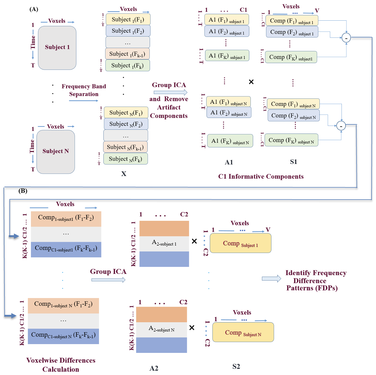
A general outline for our proposed multi-stage ICA approach is shown in Figure 1. Beginning with the application of \(K\) bandpass filters on each subject’s fMRI data, the dataset is then partitioned into \(K\) subsets, each corresponding to different frequency ranges. Let \(X^{(i)}_{k}\) denote the fMRI data matrix for the i-th subject at the k-th frequency sub-band, where \(i \in\{1, \ldots, N\}\) and \(k \in\{1, \ldots, K\}\). Subsequently, group ICA estimation⁹ is executed on the filtered data. The group ICA method is an approach to use ICA, a blind source separation method, to extract brain networks from set of data in a way that allows us to also estimate highly accurate subject specific contributions via a back-reconstruction approach that can then be used for inference.¹⁶ Group ICA is particularly useful for comparing multiple group-level IC analyses and is also applicable when combining both groups into a single group ICA framework for subsequent comparisons. This process results in the estimation of \(KC\) components (1st level components) for each dataset. This can be expressed as:

\[X_k^{(i)}=A_{1 k}^{(i)} S_k^{(i)} \tag{1}\]

Where:

• \(X_k^{(i)}\) is the observed fMRI data for subject i at frequency sub-band k,

• \(A_{1 k}^{(i)}\) is the mixing matrix (temporal components or timecourses),

• \(S_k^{(i)}\) is the source matrix (spatial components).

Some components may contain sharp edges (likely motion) or include mostly white matter or ventricles. After removing these and other artifactual components, each subject retains C1 components for each sub-band frequency (Figure 1A). To calculate FPDs, we compute voxelwise differences between each sub-band for every subject:

\[ D_{k l}^{(i)}=S_k^{(i)}-S_l^{(i)}, \text { for } k, l \in\{1, \ldots, K\}, k \neq l \tag{2} \]

where \(D_{k l}^{(i)}\) represents the difference between the components at frequency sub-bands k and l for subject i. For each subject, this results in K(K−1)/2differences, where K is the total number of frequency sub-bands.

Figure 1.A) Application of K bandpass filters to each subject’s fMRI data, partitioning the dataset into K subsets, each corresponding to different frequency ranges. Group ICA estimation is then applied to the filtered data, resulting in the estimation of C components for the dataset. After removing artifact components, we retain C1 informative components. B) Calculation of the voxelwise difference in components between sub-bands within subjects and construction of the component difference matrix (with dimensions of (k(k-1)C1/2) by voxels). Group ICA estimation is then applied to the component difference matrix. By identifying significant differences in connectivity strength, we can identify distinct spatial patterns associated with FDPs.

By applying group ICA estimation on the component difference matrix, we extract \(C2\) components (FDP components) for each component difference matrix (figure 1B):

\[ D_{k l}=A_2 S_2 \tag{3} \]

where:

• \(D_{k l}\) is the aggregated difference matrix for frequency sub-bands k and l.

• \(A_2\) and \(S_2\) are the second-level mixing and source matrices, respectively.

For each subject, the mixing matrix contains K(K-1) C1/2 values (indicating the expression of the frequency band differences for each of the first level components), and C2 components are extracted from the second ICA for each subject. Consequently, each subject has C2 FDP components.

This allows us to identify distinct spatial patterns associated with FDPs. Understanding the frequency-dependent characteristics is crucial for uncovering the underlying spatial and temporal signatures of brain activity across different frequency bands.

In this paper, we analyzed eyes-closed resting-state fMRI scans from 90 SZ patients and 90 healthy controls (HCs), obtained from the phase III dataset of the Functional Biomedical Informatics Research Network (fBIRN).³⁴ The data acquisition and preprocessing steps are explained in.²⁴ In summary, echo planar imaging was employed to acquire volumes of BOLD data across seven sites, all utilizing 3T MRI scanners. The scans were performed with an echo planar imaging sequence (FOV of 220 × 220 mm (64 × 64 matrix), TR = 2 s, TE = 30 ms, FA = 77⁰, 162 volumes, 32 sequential ascending axial slices of 4 mm thickness and 1 mm skip), and subjects kept their eyes closed throughout the scanning session. The preprocessing of the fBIRN dataset, as described in previous studies, follows a standard pipeline using the Statistical Parametric Mapping (SPM12) software. These steps included rigid body motion correction to address head motion, slice-timing correction to account for timing differences in slice acquisition and warping into the standard Montreal Neurological Institute (MNI) space using an echo planar imaging (EPI) template. Additionally, the data was smoothed to a 6 mm full width at half maximum (FWHM) using AFNI’s BlurToFWHM algorithm. This algorithm performs smoothing through a conservative finite difference approximation to the diffusion equation, a method shown to reduce scanner-specific variability in smoothness, thereby providing “smoothness equivalence” across data from multiple sites.

For this initial feasibility study, we divided the entire frequency range from 0.01 to 0.25 Hz into four equally spaced sub-frequency bands: [0.01, 0.0625], [0.0625, 0.125], [0.125, 0.1875], and [0.19, 0.25] Hz, using an 8th-order Butterworth bandpass filter for each band. This process expanded the original 180 images into 720 sub-band images. We then applied group ICA on these sub-band images, extracting 30 components (1^st level components) from each sub-band image, based on prior studies that have established 30 as an appropriate model order for identifying RSNs.

After removing components associated with sharp edges, predominantly white matter, or ventricles, we computed the frequency difference matrix by calculating within the subject voxelwise differences between components. This difference matrix was then used in a second stage of group ICA, during which we extracted 30 FDP components (2nd level components). The choice of 30 components for the second ICA was determined using the elbow method applied to a principal component analysis (PCA) scree plot. Specifically, we computed the eigenvalues of the covariance matrix derived from the second-level ICA input data and plotted the explained variance against the number of components. Using a variance threshold of 95%, the estimated number of components was found to be 30. For this stage, we included the voxelwise difference images between the four sub-bands with the components extracted from the second ICA, allowing us to investigate differences in connectivity strength between sub-frequency bands across all subjects. To evaluate the significant effects of frequency differences, we performed a paired t-test between frequency specific loading parameters for the 2^nd ICA stage. In addition, we tested for group differences within each frequency using a two-sample t-test. All statistical comparisons were conducted using the regression and t-test tools within the MATLAB software.

Group ICA was conducted using the Group ICA of fMRI Toolbox (GIFT) in MATLAB (http://trendscenter.org/software/gift).³⁵ Before applying ICA, subject-specific PCA was performed to normalize the data. The principal components from each subject were then concatenated along the time dimension, followed by group-level PCA on the combined data. The group-level principal components explaining the most variance were selected as input for the ICA to perform group-level decomposition.⁸ The Infomax algorithm was employed as implemented in the GIFT toolbox. Subject-specific time series and their associated spatial maps were calculated using a back reconstruction approach available in the GIFT software.⁸ Specifically, we used a PCA-based approach that involved reversing the forward PCA steps to project an individual subject’s data onto the group reference. This method captures subject-specific maps and time courses and has been shown to produce highly accurate individual subject information.^16,36 Bandpass filtering was executed using custom scripts within the MATLAB environment.

3. Results

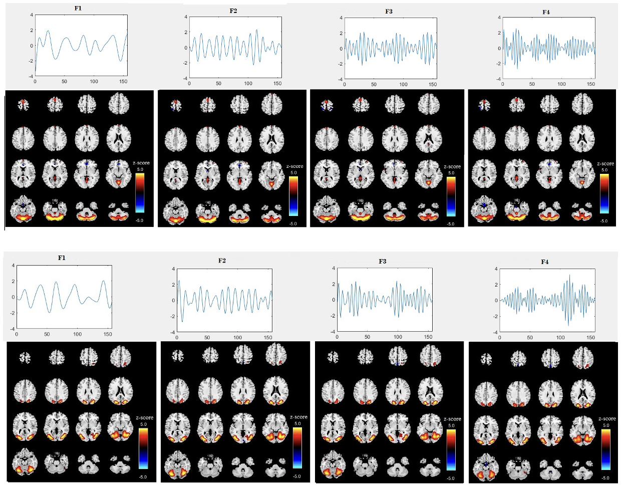
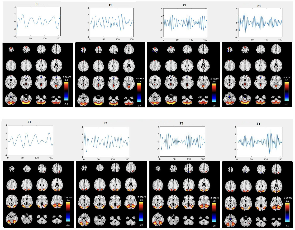
After removing components associated with sharp edges or predominantly white matter or ventricles, we were left with 24 informative components (1^st level component) (i.e. intrinsic networks). Figure 2 displays the spatial map and time course for two specific components (components 8 and 19) from the first level ICA across four different sub-band frequencies for all subjects. The time courses reveal clear differences in oscillation patterns across the frequency bands, with a transition from slow oscillations at lower frequencies (F1) to faster oscillations at higher frequencies (F4). This provides additional evidence for frequency modulation of the temporal dynamics of brain networks. The amplitude of the time courses is generally larger at the lower frequency sub-band (F1) compared to the higher frequencies (F3, F4). This is generally expected and suggests that brain activity at lower frequencies tends to exhibit more pronounced fluctuations, which aligns with the characteristics observed in certain intrinsic brain networks, such as the default mode network. The spatial maps in Figure 2 show a trend of higher voxel values in the F1 frequency band, consistent with the larger amplitudes observed at this frequency. However, there are also subtle changes in the spatial maps between frequencies, indicating that different frequency bands can highlight different aspects of brain network connectivity. The maps appear to change non-uniformly across all voxels, suggesting that these variations are not consistent throughout the brain. These spatial variations suggest that each frequency band provides unique insights into the organization of brain networks, which will be further analyzed in the subsequent ICA stage. Also, we assessed group differences in their loading parameters using t-tests, but weak p-values indicated they were insufficient for distinction. This motivated the second ICA stage to extract FDPs capturing structured frequency-specific variations.

Figure 2.The spatial map and time courses for two components from the first ICA across four different sub-band frequencies for all subjects. A display threshold of 2 was applied and the color bar represents the Z-score.

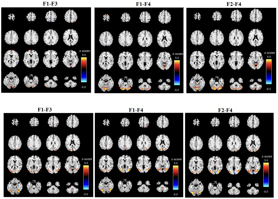
We computed the voxelwise difference of spatial maps between each sub-band frequency for each subject and then averaged the results. Figure 3 displays the results for two specific components (components 8 and 19) across two sub-band frequency differences F1-F3, F1-F4 and F2-F4) for all subjects. The differences between each sub-band frequency are clearly visible, particularly in the connectivity strength between the sub-frequency bands. This highlights the frequency-dependent characteristics of brain activity, revealing how different frequency bands modulate connectivity within the same brain networks. Although the spatial maps correspond to the same regions across sub-band frequencies, they also reveal distinct differences, highlighting variations specific to each frequency band.

Figure 3.Voxelwise difference of spatial maps between sub-band frequency F1-F3, F1-F4 and F2-F4 for two components for the first ICA stage in all subjects. A display threshold of 3 was applied, and the color bar represents the Z-score. While the overall spatial patterns are similar across sub-band frequencies, distinct differences are evident, illustrating how different frequency bands uniquely modulate neural connectivity. These findings underscore the dynamic and frequency-dependent nature of brain connectivity, highlighting the importance of analyzing sub-band frequencies to capture subtle yet significant variations in neural activity.

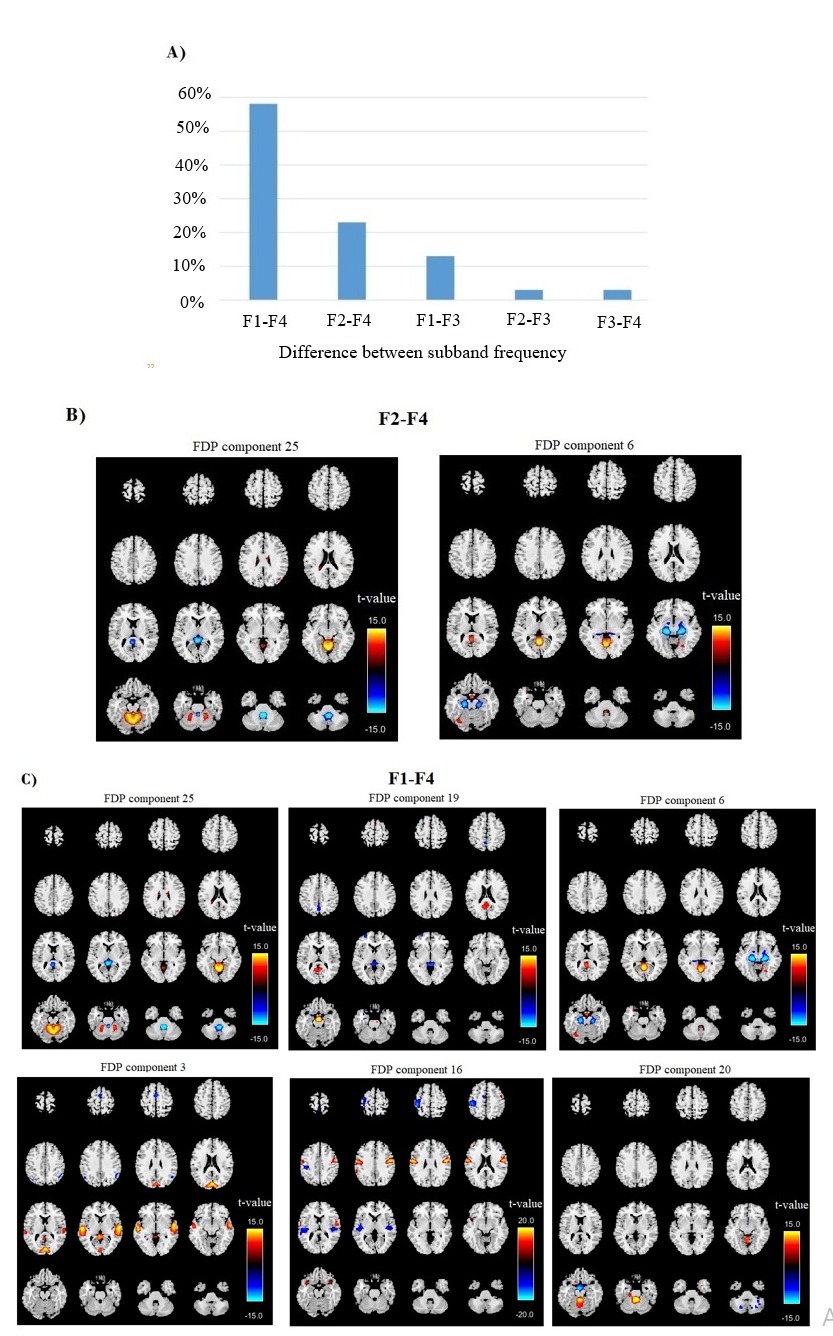
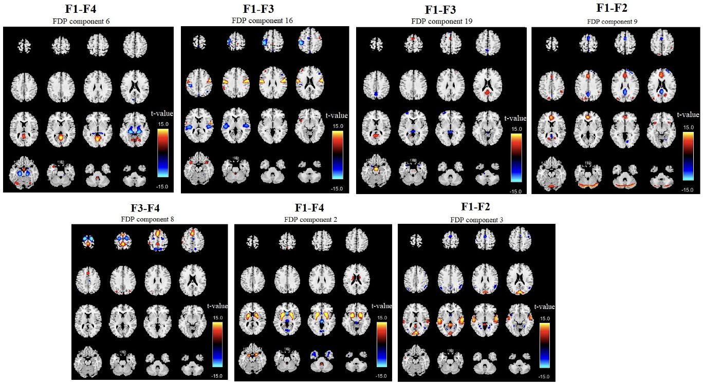
We identified FDP components that demonstrated significant differences in their loading parameters using the A2 paired t-test. Specifically, among the 180 distinct values in the loading parameters (K(K-1)C/2), significant differences were observed in 62 values with an FDR-corrected p-value < 0.01. Notably, 58% of these significant differences were related to contrasts between the F1 and F4 sub-band frequencies. Additionally, 23% of the significant differences pertained to differences between the F2 and F4 sub-bands, while 13% were associated with differences between the F1 and F3 sub-bands. Furthermore, 3% were associated with differences between the F2 and F3 sub-bands, and 3% with differences between the F3 and F4 sub-bands (Figure 4A). To emphasize the most impactful findings, we focused on the top 10% of significant results. The regions showing the most pronounced differences include the cerebro-cerebellar regions (components 6, 19, 20, 25) and cognitive control regions (components 3, 16). For these FDP components, we displayed the T-maps (Figure 4B & C), organized by differences in their sub-band frequencies. It is noteworthy that the regions exhibiting the most significant differences do not correspond exactly to standard resting-state networks; instead, they reflect spatially focal networks capturing covariation in frequency differences.

Figure 4.A) Significant differences identified by the A2 paired t-test to assess FDP variations. 58% of differences are between F1 and F4, 23% between F2 and F4, 13% between F1 and F3, 3% between F2 and F3 and 3% between F3 and F4. B) and C) FDP component T-map for the selected FDP components, displayed according to sub-band frequency differences. A display threshold of 8 was applied, and the color bar represents the T-value.

We also conducted an FDP group analysis by computing a two-sample t-test on the A2 within subject frequency differences, identifying 7 FDPs with an FDR-corrected p-value < 0.01. Figure 5 presents the T-maps of the components, organized by differences in their sub-band frequencies and sorted by t-value in descending order. The regions showing the most significant differences include the anterior and posterior cingulate cortex (FDP 9), bilateral temporal lobe (FDP 3), and basal ganglia (FDP 2), temporal lobe (FDP 8), sensorimotor region (FDP 16), anterior and posterior cingulate (FDP 9). These regions have all been previously implicated in SZ. In all cases, the t-values were positive when comparing SZ subjects to controls, indicating that SZ subjects exhibit greater frequency differences between lower and higher frequencies compared to controls.

Figure 5.Significant group differences (comparing schizophrenia subjects to controls) in FDP identified by the A2 two-sample t-test. FDP component for the 7 FDP components, displayed according to sub-band frequency differences. A display threshold of 7 was applied, and the color bar represents the T-value. The regions showing the most significant differences include the anterior and posterior cingulate cortex (FDP 9), bilateral temporal lobe (FDP 3), and basal ganglia (FDP 2), temporal lobe (FDP 8), sensorimotor region (FDP 16), anterior and posterior cingulate (FDP 9).

4. Discussion and Conclusion

In this study, we developed and applied a novel multi-stage ICA-based approach to investigate, for the first time, FDPs in resting-state fMRI data. Extracting spatial information directly from the first-level ICA across frequency bands would require voxelwise comparisons, which presents two major challenges: (1) voxelwise differences are estimated independently, making it difficult to ensure consistent behavior across the brain, and (2) this approach would involve a vast number of comparisons, increasing statistical correction challenges and computational demands. To address these limitations, we implemented a two-stage group ICA framework that focuses on FDPs, allowing for structured and interpretable comparisons of frequency-specific effects. This method involves separating fMRI images into multiple sub-frequency bands, performing group ICA to extract informative components, and computing voxelwise differences between these sub-bands for a second stage of ICA. By leveraging this design, we were able to identify distinct spatial patterns associated with FDPs, revealing significant frequency-dependent characteristics of brain activity. To demonstrate the utility of the approach, we applied this to a dataset using four frequency bands.

Our results demonstrate that RSFC is influenced by frequency-specific patterns that traditional single frequency band analyses may overlook. We initially extracted 24 informative components from the initial 30, after removing artifacts associated with sharp edges, white matter, or ventricles. Afterward, we calculated the component difference matrix and conducted a second ICA, extracting 30 components at this stage. This allowed us to explore differences in connectivity strength between sub-frequency bands across all subjects.

The differences observed suggest that certain frequency bands may emphasize or suppress specific aspects of neural connectivity. This indicates that the brain’s connectivity structure is not static but rather dynamically varies depending on the frequency band being analyzed. The spatial distribution of these differences reveals subtle yet important variations in connectivity patterns, emphasizing the need to consider sub-band frequencies when analyzing brain connectivity. These differences motivate our FDP approach to extract multivariate frequency specific networks to capture these nuanced variations. This approach will provide a useful decomposition of the BOLD fMRI signal and may prove useful in further illuminating the underlying mechanisms of brain activity and how different frequency bands contribute to the overall functional architecture of the brain.

Our paired t-test on the A2 loading parameters uncovered significant frequency-dependent differences in connectivity strength between sub-frequency bands in FDPs, shedding light on the nuanced characteristics of brain activity across these frequencies. Specifically, the T-maps in Figure 4 highlight distinct spatial patterns in networks extracted from the F1-F4 and F2-F4 sub-bands, revealing that the frequency-specific RSFC patterns are not uniform. Notably, the regions exhibiting the most significant differences do not align precisely with standard resting-state networks; instead, they reflect spatially focal networks that capture covariation in frequency differences. This suggests a much more complex relationship between frequency and connectivity, motivating additional work focused on characterizing these multivariate relationships and linking them to potential mechanisms.

Our work also shows that FDPs have significant relationships with mental illness. Specifically, the A2 two-sample t-test revealed significant group differences in FDPs, highlighting how brain connectivity varies in SZ across different frequency bands. The most striking variations were observed in regions such as the cerebellum, cingulate cortex, temporal lobes, basal ganglia, and sensorimotor regions. These findings align with previous research indicating that these areas are critically involved in the neuropathology of SZ. For instance, the altered connectivity in the cerebellum and cingulate cortex reinforces the idea that SZ involves disruptions in both motor coordination and cognitive control networks.^37,38 Similarly, the observed differences in the temporal lobes and basal ganglia further support their established roles in auditory processing and motor function, both of which are often impaired in SZ.^39,40 Garrity et al.⁴¹ similarly reported that SZ is associated with altered temporal frequency and spatial location of the default mode network.

Additionally, HC subjects showed significantly more power in low-frequency oscillations (0.03 Hz), whereas patients with SZ exhibited more power in higher frequencies (0.08 Hz to 0.24 Hz). Our findings are consistent with, but significantly extend, these observations, as we also identified significant differences between SZ and HC in both high and low frequencies, suggesting that these two groups exhibit greater differences at these extremes. Calhoun et al.⁴² also demonstrated that SZ patients show changes in posterior default mode regions, which is corroborated by our results in Figure 5, where the most significant changes were observed in these areas. Fryer et al.⁴³ also identified differences between SZ and HC in regions such as the posterior cortex, occipital lobe, and cerebellar lobes. These observations have been supported by other studies.^44–48 However, our multi-frequency band approach extends this work by highlighting multivariate patterns of frequency change, offering a more nuanced understanding of the frequency-dependent characteristics of brain activity in SZ.

5. Limitations and Future Directions

Our frequency-specific analysis identifies patterns that appear to correspond to distributed and often bilateral networks, suggesting that RSFC is a multi-frequency band phenomenon, with each frequency band contributing uniquely to the brain’s functional architecture. This has important implications for future research, as it indicates that exploring frequency-specific RSFC can uncover connectivity patterns not apparent in single-frequency band analyses. Understanding these patterns may be crucial for elucidating the underlying mechanisms of brain function and dysfunction.

Our study introduces a comprehensive method for analyzing frequency-specific RSFC using a multi-stage ICA approach. The significant frequency-dependent and group-specific connectivity patterns we identified highlight the importance of considering multiple frequency bands in fMRI analyses. These findings open new avenues for investigating the brain’s functional architecture and its relation to cognitive processes and psychiatric disorders.

Future work should focus on validating these findings in larger and more diverse cohorts and exploring the clinical relevance of frequency-specific RSFC patterns. Additionally, while we focused on low-model-order ICA in this project, future research should explore ICAs across a range of model orders. The spatial scale of ICNs can be effectively controlled by adjusting the model order of ICA, enabling the study of brain segregation and ICNs estimation at different spatial scales.⁴⁹ Low-model-order ICAs result in large-scale, spatially distributed ICNs,^50,51 while higher model orders yield more spatially granular ICNs.^16,48,52 In Iraji et al.,²⁶ they proposed using multi-scale ICA (msICA), which involves running ICA with multiple model orders, to estimate functional sources across multiple spatial scales.

Moreover, while ICA was chosen due to its ability to capture higher-order statistical dependencies and provide a soft clustering approach, future research should investigate alternative clustering methods for FDP estimation. Comparing ICA with techniques such as hierarchical clustering, k-means, or graph-based clustering could provide additional insights into the best approach for identifying frequency difference patterns. It would also be helpful to explore approaches to optimize the FDP estimation using other types of statistical diversity to help enhance our understanding of FDP structures.

Additionally, integrating our approach with other imaging modalities and exploring its applicability to different cognitive tasks and conditions can further enhance our understanding of the brain’s complex functional networks. Our approach offers a powerful tool for advancing neuroimaging research, providing a deeper and more detailed perspective on the brain’s functional connectivity. We anticipate that this method will significantly contribute to the field, offering new insights into the spatial and temporal dynamics of brain activity across different frequency bands.

Finally, our methodology currently divides the 0.01–0.25 Hz range into four equally spaced sub-frequency bands. Future work should assess the sensitivity of results to this parameter by testing different numbers of sub-bands or ranges. Ideally this choice could be optimized by the algorithm, a topic we hope to explore.

Data and Code Availability

Due to IRB restrictions, data cannot be shared directly; however, inquiries can be directed to tvanerp@hs.uci.edu.

Funding Sources

The authors acknowledge funding from the following grants: NSF 2112455 and NIH R01MH129493.

Conflicts of Interest

The authors declare no competing interests.