Understanding variability in brain MRI templates: Optimal sample sizes for representative population averages

Introduction

Automated image processing in neuroanatomical and functional studies predominantly relies on average anatomical templates as targets for registration to compare data over subjects and between groups. Over the past two decades, numerous anatomical templates have been developed and made accessible to the scientific community. Our group has created a number of human brain templates¹ that have been incorporated into open image analysis tools like FreeSurfer,² SPM,³ and FMRIB⁴ to define the target stereotaxic space.⁵ Other groups have also created and made available multiple different anatomical templates for the scientific community using variable methods. A recent paper describes TemplateFlow, a web-based repository containing 25 brain templates.⁶ Table 1 lists some of the most popular templates.

A common assumption in the creation of average anatomical templates is that the average template is an optimal registration target, allowing the “smallest” parametrization for mapping of each MRI scan in the population into a common coordinate system.^11,16 It has been shown^7,17 that the template which minimizes the average distance (or bias) from all population subjects satisfies these requirements. Such an anatomical template is also called “unbiased”, which will be the definition used in this paper.

The number of subjects used to create these average templates often depends on what is available. It remains unclear how many subjects are necessary to capture population variability effectively and produce truly representative, unbiased averages of brain anatomy. Key considerations include the design constraints of templates, such as computational requirements and the availability of the software. Additionally, the methods used for registration and the strategy employed to generate the templates are crucial factors. Other considerations include the intended purpose of templates, which is to facilitate cross-time, cross-subjects, and between-group comparisons. They should also enable accurate registration within studies while minimizing bias. The notion of a minimum deformation target, as discussed by Ashburner,¹⁸ underscores the importance of reducing bias in template construction.

Recently, Yang et al.¹⁹ performed an experiment to determine the optimal number of subjects needed to create a stable population average, using two cohorts: a young Caucasian population from the Human Connectome Project²⁰ (n=800 subjects, 22–35 years old) and a young Chinese population (n=250 subjects, 19–37 years old). They used random subsamples with a variable number of subjects, ranging from 20 to 400, to generate population averages and then estimated variability of the resulting population templates depending on the number of subjects and race.

In this study, we experimentally investigate the impact of the number of subjects on the creation of unbiased population templates using data from the UK Biobank²¹ with a much larger number of subjects. In addition, to ensure generalizability of results, we compare two existing algorithms widely used to generate an unbiased population average: ANIMAL⁷ and ANTs,¹¹ with the aim of determining the number of subjects required for each algorithm to achieve a stable population average.

In a hypothetical ideal situation, if a truly unbiased template were available for the whole study population, we would use it as a “gold standard” reference to compare against templates generated from a subset. Given practical considerations such as computation time, we generated two unbiased templates from 2000 subjects to use as “silver standards” to estimate quality metrics for both methods. Our findings indicate the point at which increasing the number of subjects no longer significantly reduces the variability of results, thereby providing insights into the optimal subject count for template creation.

Materials and Methods

Materials

We used MRI scans of the human head available from the UK Biobank.²¹ At the time of writing, we had access to the scans of 39677 subjects from version v14940, with mean age of 54.8±7.5 years old. All images were scanned using the same scanner type, a Siemens Skyra 3T, with a 3D MPRAGE sequence (TR = 2000 ms, TE = 2.01 ms, TI = 880 ms, and flip angle = 8°) and 1 mm x 1 mm x 1 mm voxels. All 39677 MRI brain volumes were preprocessed using the pipeline described below. All resulting images were evaluated by automated QC.²² From the 33725 that passed automatic stereotaxic registration QC, we selected a random subset of 2000 scans (1000 M, 1000 F) of subjects between 40 and 60 years old. See Table 2 below for study population statistics.

Ethics

Written informed consent was obtained from all UK Biobank participants (see “UK BIOBANK ethics and governance framework”). Research ethics approval was obtained from the North West Multi-centre Research Ethics Committee (for details see https://www.ukbiobank.ac.uk/learn-more-about-uk-biobank/about-us/ethics).

Methods

Preprocessing

We downloaded raw T1w scans from the UK Biobank repository and pre-processed them using the following steps:

• Intensity non-uniformity correction using N4, parameters: distance 100 mm, iterations: 200x200x200x200,0.

• Histogram-based linear intensity scaling, by matching histogram to that of the MNI-ICBM152 2009c template.

• Linear stereotaxic registration to MNI-ICBM152 2009c space using the improved bestlinreg algorithm.²³

• Automated quality control of the linear registration using DARQ.²²

Registration

To ensure generalizability of results, we compared two template building algorithms for the generation of unbiased population templates: The first is based on ANIMAL⁷ and the second, on ANTs.¹¹ Both methods have been used in the literature for construction of several widely used population templates.

In short, both algorithms work by iteratively estimating minimum-deformation templates from a set of MRI scans. The two methods are described below.

ANIMAL-based⁷

Uses ANIMAL²⁴ to perform non-linear registration. Each scan is registered to the current estimate of the template at a given level of detail. The average inverse transform is calculated and concatenated to each individual transformation. The resulting transformation is applied to resample the scan in template space. All warped scans are averaged to create a new unbiased template estimate. These steps form one main iteration. These iterations are repeatedly performed with reducing levels of detail, starting at 16 mm steps for non-linear deformation to address the largest deformations, and ending with 2 mm steps to refine anatomical details. We used normalized cross-correlation as a cost function and the current implementation of the ANIMAL-based template building, available as part of “NIST-MNI image processing pipelines” (https://github.com/niST-MNI/nist_mni_pipelines).

ANTs¹¹

Uses ANTs Greedy SyN method.²⁵ Each scan is registered to the current estimate of the template and warped to match the template. All warped scans are averaged, and average non-linear transformation is calculated. The inverse average non-linear transformation is then calculated and scaled by a gradient step and applied to warp the average to create the new unbiased template estimate. The ANTs template building script applies Laplacian sharpening after averaging individual co-registered scans, resulting in a further increase of the sharpness. See the source code of AverageImages tool from ANTS toolkit, line 147 (https://github.com/ANTsX/ANTs/blob/master/Examples/AverageImages.cxx#L147). This process is repeated iteratively, each time at the highest level of detail (1 mm steps). We used a locally normalized cross-correlation cost function and the script “antsMultivariateTemplateConstruction.sh”, included with the ANTs software package (https://github.com/ANTsX/ANTs), with parameters from.¹¹

Differences between the two methods (ANIMAL vs. ANTs) for template creation

There are several important differences between the two registration methods:

• Registration method:

  • ANIMAL uses local Simplex optimization to find deformation vectors optimizing local similarity between corresponding patches. The overall transformation is regularized by applying Gaussian smoothing to these vectors. These steps are repeated for a fixed number of iterations. Inverse deformations are calculated using local Newton optimization. There is no explicit constraint on invertibility of the deformation field or its inverse-consistency.

  • ANTs uses a greedy symmetric normalization algorithm, calculating forward and inverse transformations simultaneously, which are guaranteed to be inversely consistent.

• Interpolation method:

  • ANIMAL uses 3rd order b-spline interpolation to resample each MRI before voxel-wise averaging to build the template at each iteration.

  • ANTs uses 2nd order b-spline interpolation.

• Iterative scheme:

  • ANIMAL uses a hierarchical scheme, where a minimal deformation template is estimated first at a coarse level of detail, then more refined at each iteration, and so on. In short, at the first main hierarchical step, a 16 mm deformation is estimated for all subjects, and this data is used to generate a 16 mm template average. This process is repeated 4 times to build the final 16 mm template. The final 16 mm template is then used as the target for an 8 mm non-linear deformation estimate for all subjects using the same strategy. This process is repeated until a 2 mm deformation model is created.

  • The ANTs method uses a fixed level of detail and hierarchical scheme at the individual registration level only (e.g., at each iteration, each subject is registered at a 1 mm deformation grid to the current estimate of the unbiased template).

• Final level of registration detail:

  • The ANIMAL method stops at a 2 mm step size for the deformation grid.

  • The ANTs method performs registration down to 1 mm steps.

Experimental setup

The following steps were repeated with both ANIMAL and ANTS methods:

• We created a single unbiased population average using all 2000 scans to be used as a silver standard template. With such a large number of subjects, we hoped to build a sample mean that would be very close to the population mean. We then estimated a deformation field T_i,ss mapping each subject i into a common silver standard space (ss), and a deformation field R_i,ss reverse mapping from common space into each subject’s space. These silver standard deformation fields, one from ANIMAL and one from ANTS for each subject, serve as the reference for the analysis below (See Fig. 1.1).

• We randomly chose N=[10, 20, 40, 80, 160, 320] samples to evaluate template creation with different numbers of subjects. We repeated each template creation experiment 50 times for each value of N, drawing new samples (without replacement, without maintaining sex balance from the 2000 scans used to build the silver standard) for each iteration k. After each experiment, we again obtained forward and backward transformations: T_i,k and R_i,k. The rationale for not using sampling with replacement, as commonly done in bootstrapping experiments, is that it is virtually impossible to have two subjects with identical folding pattern, therefore sampling with replacement would create an unrealistic population sample.

We use the following formula to calculate the distance between each transformation and a silver standard transformation:

D_i,k = R_i,ss ∘ T_i,k,

where ∘ represents concatenation operator. Here D_i,k represents a non-linear transformation that can be represented as a dense vector field, defined at each voxel of the silver standard template space, where each vector represents a misregistration “error” between registration parameters of the subject I in the experiment k from the silver standard (See Fig. 1.1, 1.2). This error can be characterized in several different ways:

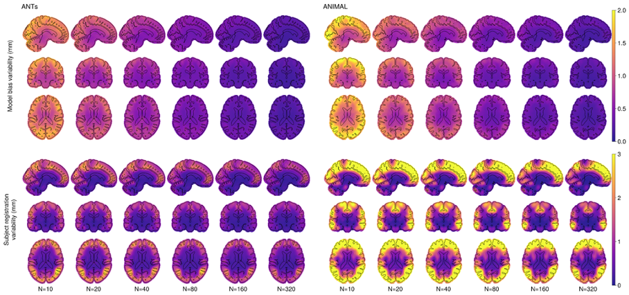
1) Model bias variability: mean D_i,k for each experiment k—showing a mean shift between the silver standard and the subset, followed by standard deviation across all subsets. This metric represents the variability of the k-th average template’s overall shape relative to the silver standard.

2) Individual subject registration variability: standard deviation of D_i,k followed by the average across all subsets. This metric represents variability of the individual transformations to obtain the unbiased template k.

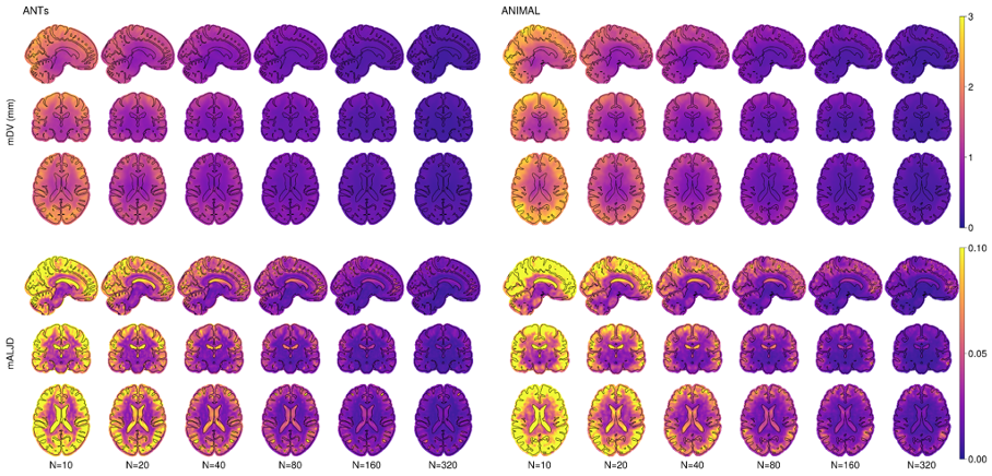
3) Mean deformation value (mDV): as introduced in¹⁹ is the mean Manhattan distance of the voxel’s displacement distance between silver standard and each template k.

4) Mean absolute logarithmically transformed Jacobian determinant (mALJD): as introduced in¹⁹ is a mean of the absolute log-Jacobian of the displacement between the silver standard and each template k.

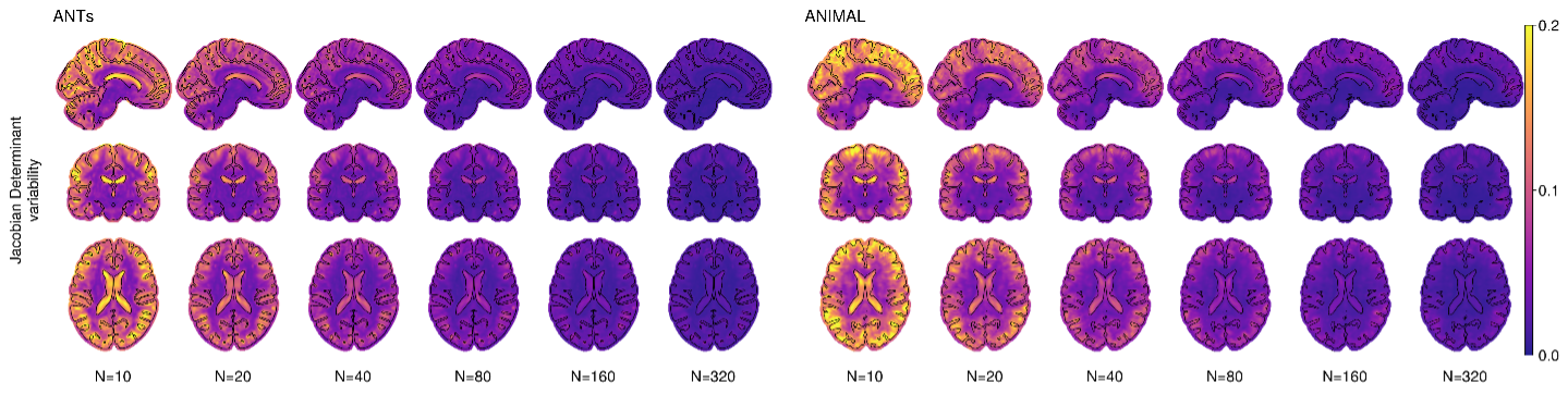
5) Jacobian determinant variability (JDV): is the standard deviation of the Jacobian determinant of D_i,k across all subjects in the subset, averaged across all subsets. The Jacobian determinant is a ratio of the local volume change, meaning that value of 0.1 corresponds to the 10% volume change. This metric shows variability of the local Jacobian determinant and can be used to estimate the local effect size for the power calculation as the denominator in Cohen’s d formula in cross-sectional analysis.

Overlap metric

We used SynthSeg²⁶ to segment each T1w scan into 32 anatomical regions. We chose this method because it does not depend on registration, and the authors showed high reproducibility and robustness of this method. We used the generalized overlap ratio metric¹⁷ to quantify the accuracy of co-registration of different MRI scans used to create each template, then we averaged (voxel-wise) between experiments for each N, creating intra-template overlap maps. We also performed voxel-wise majority voting of each template to generate template segmentation and then calculated voxel-wise overlap ratio between different templates (“inter-template” overlap maps). This results in two additional evaluation metrics:

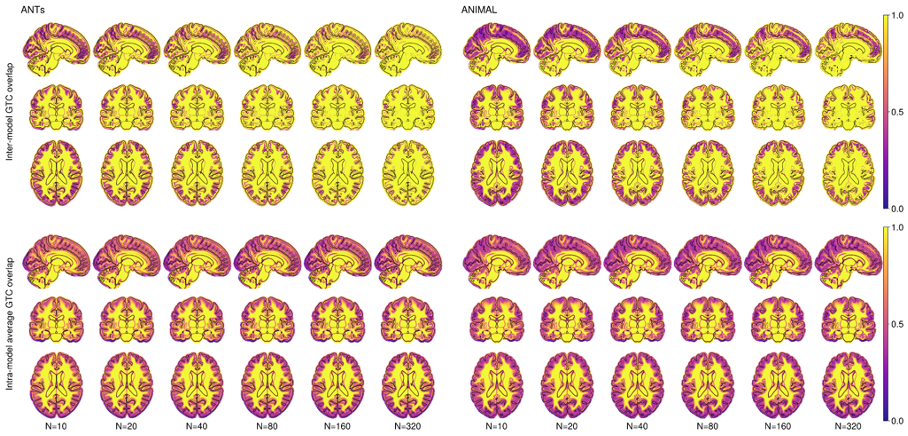
6) Inter-model generalized Tannimoto coefficient (GTC) overlap: showing degree of concordance of the segmentation results between templates.¹⁷

7) Intra-model average GTC overlap: average GTC overlap for individual segmentations inside each model that shows the overall degree of consistency of co-registration of subjects with each model.

Convergence analysis

Similarly to methods previously proposed¹⁹ we calculated metrics for model bias variability, subject registration variability, mDV and mALJD on a region-of-interest (ROI) basis, and fit a power function to estimate the number of subjects that would be needed to achieve convergence of the template building algorithm, depending on the area of interest that is being studied. We used the following definition of the convergence, similarly to¹⁹: the number of subjects that are required to achieve below 5% of the slope of the 1st derivative of the power function with respect to the slope for 20 subjects. This means that to achieve a decrease in the metric, the number of subjects that needs to be added to the model is 20 times more than when only 20 subjects are used.

Power Analysis Application

Calculating the JDV allows us to perform power analysis for deformation-based morphometry (DBM) in a sense of estimating minimal detectable difference for a hypothetical cross-sectional experiment, with 50/50 split between two groups of subjects, where population average is obtained using either the ANTs or ANIMAL methods, followed by statistical analysis of the Jacobian determinants of the resulting deformation fields. We sampled values of the JDV metric in several anatomical ROIs and fit the same power function as described above to estimate JDV for different values of N. Then, using the sample-size Lehr equation²⁷ we estimated the minimal detectable difference between two groups of subjects with 50/50 split between groups with α =0.05 and 80% power in a hypothetical cross-sectional experiment:

\[n \approx 16\frac{s^{2}}{d^{2}}\]

where d is expected difference between mean values of two samples, and n is the number of samples in each group.

Results

Qualitative Results

Figures 1.1 and 1.2 show examples of the unbiased averages for N=10, 20, 40, 80, 160, 320 and 2000 scans from the UK Biobank, using ANTs¹¹ and ANIMAL.⁷ While not the true population mean, the N=2000 silver standard is assumed to be quite close. One can see that for N <80, there are evident anatomical differences (see arrows Fig. 1.2) with the silver standard for both ANTs and ANIMAL averages. These images indicate that N < 80 is not enough to be representative of the population average.

Figure 1.1.Unbiased averages for N=10, 20, 40, 80, 160, 320 and 2000 UKBB scans using ANTs (top row) and ANIMAL (bottom row). Arrows draw attention to anatomical differences with the silver standard.

Figure 1.2.Unbiased averages for N=10, 20, 40, 80, 160, 320 and 2000 UKBB scans using ANTs (top row) and ANIMAL (bottom row). Closeup view. Arrows draw attention to anatomical differences with the silver standard. Recall that ANTs template building uses a Laplacian sharpening step. This might explain the higher apparent edge contrast in the ANTs templates.

Figure 1.3 shows an example of the inter-model variability when a small number of scans are used to calculate the averages. Again, arrows in the figure draw attention to the differences.

Figure 1.3.Individual examples of unbiased averages for N=10 UKBB scans using ANTs (top row) and ANIMAL (bottom row). Closeup view.

Quantitative Results

Voxel-level Quantitative Results

Figure 2.1 shows the model bias variability and subject registration variability on the voxel level. As expected, there is higher variability at the cortex compared to the deep brain, which decreases with increasing N. The positional variability (i.e., the mismatch with the N=2000 silver standard depending on the anatomical ROI) is minimized using 80 or 160 subjects when using ANTs. The ANIMAL-based unbiased average requires N=160 to achieve a similar result. Interestingly, individual positional variability (i.e., the anatomical variability between subjects) stays roughly the same for all N of both methods.

Figure 2.1.Model bias variability (top) and individual subject registration variability (bottom) for ANTs (left) and ANIMAL (right) methods for N= 10, 20, 40, 80 160 and 320 subjects.

Figure 2.2 shows the mDV and mALJD. In general, the mDV reinforces the model bias variability, with the difference being the use of Manhattan distance instead of Euclidean distance for characterizing local variability of shape. As such, the same comment as above applies here. The mALJD reflects a different aspect of the model variability: rather than showing displacement in mm, it represents variability of the local volumes. Surprisingly, even though the mDV metric demonstrates a noticeable difference between ANIMAL and ANTs, the mALJD metric shows that there is a little difference between the two methods, although for the small number of subjects (below 20), ANTs seem to produce slightly less variable results.

Figure 2.2.Mean deformation value (mDV, top) and mean absolute logarithmically transformed Jacobian determinant (mALJD, bottom) for ANTs (left) and ANIMAL (right) methods for N= 10, 20, 40, 80 160 and 320 subjects.

Figure 2.3 shows the average Inter-Model GTC overlap and average Intra-Model GTC overlap, also on a voxel level. These measures show how well segmented anatomical structures co-register together. As expected, there is higher variability at the cortex compared to the deep brain, and this variability decreases with increasing N.

Figure 2.3.Inter-model overlap (top) and intra-model overlap (bottom) for ANTs (left) and ANIMAL (right) methods for N= 10, 20, 40, 80 160 and 320 subjects.

Figure 2.4 shows the JDV at voxel level. This parameter can be used as the denominator in Cohen’s d effect size formula for the power calculation in hypothetical cross-sectional analyses.

Figure 2.4.Jacobian determinant variability estimated for ANTs (left) and ANIMAL (right) methods for N= 10, 20, 40, 80 160 and 320 subjects.

Convergence analysis result and region of interest level quantitative results

Results of the convergence analysis are shown on Figure 3.1 and Figure 3.2, where the fitted functions and red numbers indicate the estimated number needed for convergence. Adding more subjects yields diminishing improvements in model stability. The number of subjects required for model bias variability are similar between ANTs and ANIMAL methods. However, more subjects are required (roughly 2x) for ANIMAL to achieve equivalent subject registration variability. The mDV and mALJD are very similar between methods.

Figure 3.1.Model bias variability and individual subject registration variability for both unbiased template registration methods computed for different brain regions. The brain stem, deep grey matter nuclei, and ventricles show the lowest average position variability, and cortical grey matter the highest. Values for model bias variability are similar for ANTs and ANIMAL methods. Roughly half as many subjects are required for ANTs to achieve equivalent subject registration variability.

Figure 3.2.Inter-model overlap and intra-model overlap for both unbiased template registration methods computed for different brain regions. The brain stem, deep grey matter nuclei, and ventricles show the lowest average position variability, and cortical grey matter the highest.

Figure 3.3.Mean deformation value (mDV) and mean absolute logarithmically transformed Jacobian determinant (mALJD) for ANTs (left) and ANIMAL (right) methods for N= 10, 20, 40, 80 160 and 320 subjects. These metrics show surprisingly similar results across all structures, except for the brainstem in ANTs, where the method converges with more subjects.

Power analysis results

Figure 3.4 shows the results of the power analysis estimation of the minimal detectable difference between two groups of subjects with 50/50 split between groups with α =0.05 and 80% power in a hypothetical cross-sectional experiment. Note that the y-axis is shown on a log-scale and units are the percent of the local difference between two groups of subjects.

Figure 3.4.Estimation of the minimal detectable difference (in percent) for hypothetical deformation-based morphometry experiment shown on a log-scale for ANTs (left) and ANIMAL (right) methods for N= 10, 20, 40, 80 160 and 320 subjects. Here it is visible that ANTs allows detection of a given difference using a slightly smaller number of subjects.

Discussion

In this paper, we have built the largest (N=2000) unbiased average template MRI brain model to use as a silver standard of the average brain shape. We used data from the UK Biobank—high quality, high resolution, high contrast T1w MRI data from subjects with a broad age range, acquired on identical scanners that enabled us to focus on anatomical differences and not scanner differences. Our comparative experiments demonstrate that both methods, ANTs and ANIMAL, can successfully build unbiased average templates.

The quantitative results show that as far as the shape of the average template is concerned, the ANTs method achieves smaller variability of the overall shape of the template for a given number of subjects. This is particularly noticeable in the cortical regions, where inter-subject variability is reduced by a factor of two with the ANTs method. Figure 3.1 shows that for inter-subject registration variability estimated in the cortical grey matter (GM) ROI, the ANTs method converges after 240 subjects with remaining variability of roughly 1 mm, whereas the ANIMAL method converges after more than 400 subjects, with residual variability of approximately 2 mm. This is perhaps due to two reasons. First, the ANTs registration algorithm runs to 1 mm deformation field step size, whereas the ANIMAL method stops at a rougher resolution of 2 mm. Second, ANTs uses symmetric normalization of the deformation fields, while ANIMAL uses simple Gaussian blurring of the deformation fields for regularization.

Apart from the geometric measurements derived from the registration parameters of the silver standard, we have tried to estimate goodness of co-registration by measuring degree of agreement of segmentations between models. We use the overlap metric as another proxy of the goodness of the model.

The inter-model overlap metric plotted in Figure 3.2 shows that with an increased number of subjects, the overlap gradually reduces in the cortical GM ROI, for both ANTs and ANIMAL, possibly indicating that neither of the proposed methods is able to fully capture the anatomical variability of the cortical folding pattern. Another potential possibility is that voxel-based non-linear registration methods like ANTs and ANIMAL are not sufficient to co-register cortical gyri and sulci and surface-based methods should be used instead when accurate cortical co-registration is needed.

Interestingly, both methods converge to a stable population average when measured with residual model bias variability of ~ 0.25 mm and mDV of ~ 1 mm after roughly 160 iterations in all regions of the brain (see model bias variability in Figure 3.1, and mDV in Figure 3.3). The only exception is for the brainstem and cerebellar white matter (WM), where ANTs surprisingly needs more than 200 subjects to converge to a stable population average.

The JDV metric (Figure 2.4) can be used to estimate the smallest possible effect size that can be captured reliably when non-linear registration methods are used for DBM experiments to determine the minimal effect size that can be reliably captured. This metric could be used to help estimate the required number of subjects in a power calculation for pharmaceutical trials that target specific brain regions.

Our findings are consistent with those published in ¹⁹, which showed that 200 subjects are enough to achieve a stable population average, although using a smaller population pool and using a single template building algorithm (ANTs).

Our power analysis estimations show one of the practical applications of the result of this study: estimating minimally detectable change for statistically significant result at α =0.05 with 80% power in a hypothetical DBM experiment, or alternatively one can estimate required number of subjects for an expected difference between two populations, depending on the anatomical location. Results show that ANTs has a slight advantage over ANIMAL with regard to the number of subjects required to detect a given difference, especially in the cortical GM. Also, clearly visible is that a smaller number of subjects would be needed in deep GM, brainstem, and cerebellar WM structures than anywhere else.

Our paper is not without limitations. First, while we only compared ANTs and ANIMAL algorithms, we would expect similar results with other unbiased average template creation strategies. Second, we ran ANIMAL using default parameters that estimated the final deformation grid at a 2 mm spacing, potentially limiting its performance in comparison to the ANTs deformation grid at 1 mm spacing. Third, the ANTs method includes a Laplacian sharpening step that increases the GM:WM contrast in the average template. This may give an advantage to the ANTs strategy where non-linear registration of a subject benefits from the sharper edges in the unbiased average template target at each iterative step. Fourth, SynthSeg was used to segment regions in each subject’s MRI. Any errors in segmentation will confound our inter- and intra-model overlap metrics used to estimate quality of registration. These confounds should affect ANTs and ANIMAL in a similar manner and not result in a bias between registration methods. In addition, inclusion of more subjects increases subject variability as the potential for contradictory anatomical information will reduce overlap and increase blurring. Fifth, our silver standard template is good, but not perfect. Since N=2000 is large, and we took care to include equal numbers of cognitively normal men and women, it should yield a good estimate of the population mean. However, these 2000 subjects were selected from the UK Biobank, which is already a subsample UK population only above 40 years of age. As seen from Table 2, 98% of the participants are white, and 84% are born in England. We expect our results to generalize to other healthy populations, but further experiments are needed to confirm this. We would also expect different numbers needed to achieve a stable population average when a diseased or more diverse population is being studied.

Neither ANTs nor ANIMAL can fully capture cortical variability—neither method can unfold the cortical anatomy of one subject to refold it to fit the gyral and sulcal pattern of another subject (or template). This suggests that surface-based methods may be better at precise cortical alignment to model the average cortex. While this might be possible for the primary and many secondary gyri and sulci, it is not clear that all secondary and tertiary gyri and sulci can be aligned because there is not a one-to-one homology across cortices for all subjects. In future work, it might be interesting to classify subjects into a particular cortical folding pattern for a specific sub-region of the cortex, and then average only subjects with the same folding pattern—but only for that specific region.

Conclusions

Our goal was to determine, within the population represented by the UK Biobank, what is the minimal number of subjects required to generate a stable average, where adding more subjects does not significantly improve the estimate of the average shape. In future work, it would be interesting to see if our results hold for sub-populations: for example, for men vs. women, for subjects with different neurodegenerative diseases such as Parkinson’s or Alzheimer’s disease or for adolescents with attention deficit hyperactivity disorder. One might hypothesize that for some disease-specific population templates, more subjects might be necessary due to added variability from disease, in addition to naturally occurring anatomical variability between subjects.

Our experiments show that 160 samples are sufficient to achieve a stable population average with both template building methods. However, if a smaller number of samples are available, ANTs achieves stable results with a smaller number of samples in most brain regions. Stability of the population average varies spatially, and neither method fully captures anatomical differences in the cortical folding patterns, indicating that surface-based or hybrid methods should be developed for the tasks where accurate cortical co-registration is needed. The silver standard average templates are available at: https://nist.mni.mcgill.ca/uk-biobank-average-2000/.

Data and code availability

Data used in the research are available from the UK Biobank: www.ukbiobank.ac.uk. The final versions of the generated templates are available at https://nist.mni.mcgill.ca/uk-biobank-average-2000/. Code used to generate average templates and to perform statistical analysis is available upon reasonable request.

Acknowledgements

This research has been conducted using the UK Biobank Resource under Application Number 45551.

This research used the NeuroHub infrastructure and was undertaken thanks in part to funding from the Canada First Research Excellence Fund, awarded through the Healthy Brains, Healthy Lives initiative at McGill University.

This research was enabled in part by support provided by Calcul Québec and the Digital Research Alliance of Canada.

We acknowledge the help of Dr. Stanley Hum, with editing the manuscript.

Funding Sources

Authors received funding from Famille Louise & André Charron and Canadian Institutes of Health Research (MOP-111169).

Conflicts of Interest

Authors have no conflicts of interest to disclose.