Data-guided neuroimaging and visualization: From functional decomposition to dynamic fusion

Introduction

The brain mapping community remains vibrant and rapidly evolving, with the Organization for Human Brain Mapping (OHBM) serving as a catalytic force for discovery and innovation. The pace and breadth of progress continue to be both inspiring and, at times, dizzying. In this article, I reflect on several themes that I return to often–topics that I believe are central to ongoing research in our field. These reflections are grounded in both personal experience and current methodological trends, and I offer examples from my own work to help stimulate continued discussion and development.

As a researcher immersed in neuroimaging methodology, I’ve found that clarity and innovation often arise from adhering to a core principle: staying close to the data. This means resisting the temptation to impose early, low-dimensional summaries and instead embracing the full complexity of high-dimensional data. Data-driven approaches have repeatedly revealed unexpected patterns and relationships–insights that often precede and inspire new theoretical models. Over the course of my career, I have worked to bridge these data-driven discoveries with structured, model-based frameworks, aiming to combine exploratory richness with interpretive rigor. This balance has proven crucial for advancing our understanding of both healthy brain function and clinical dysfunction.

The paper is organized around six interconnected topics. I begin with two focused on data decomposition: first, I introduce a conceptual framework for categorizing spatiotemporal decompositions of brain data; second, I highlight the promise of data-driven and hybrid models for capturing both inter-individual variability and dynamic spatial patterns. The next two topics explore the use of independence and higher-order statistics in disentangling relevant features, followed by a discussion of expressive visualization–a paradigm for surfacing complex patterns within modern NeuroAI models. Finally, I turn to two emerging areas: recent developments in modeling brain dynamics and advances in symmetric, multimodal and dynamic fusion. Together, these topics outline a vision for methodologically rigorous and expressively rich brain mapping in the years ahead.

Functional decomposition framework

The brain is a spatiotemporal organ. Decomposing or representing such data are a key aspect of neuroimaging work. One can choose from fixed, anatomic or connectome-based atlases¹ to capture pre-determined boundaries, adaptive, data-driven components to better capture individual variation,^2,3 approaches that have elements of both.^4–6 One can consider the use of an atlas as a specific type of “functional decomposition”, a term I next define in a more general sense. Currently there are dozens of atlases one can select from, and, more recently, computational and ontological tools for translating between atlases.^7–9 Beyond this, selecting between surface or voxel space and which atlas to use can have an outsized impact on the results. Data-driven approaches have been widely used as well, but these are typically derived for a given study.

The strength of data-driven approaches is that they can better fit the data, leading to a more faithful representation of the underlying patterns. However, a limitation of the data-driven approach is that it can be challenging to find correspondence among subjects or studies that use fully data-driven approaches. This was the motivation for the widely used group independent component analysis (ICA) approach,¹⁰ that is, to allow for correspondence between single-subject spatial maps and timecourses within an ICA model. The same principle can be applied to the use of more complex neural network decompositions, which tend to focus either on single subject models or group level models.¹¹ We can leverage a two-step project to capture both group and subject-specific neural network decompositions that can capture nonlinear relationships while also providing subject specific information.¹² Hybrid approaches, such as the NeuroMark pipeline^5,13,14 discussed in the next section, leveraging spatial priors,¹⁵ represent a natural trade-off between fixed atlases and data-driven solutions as they provide correspondence between subjects, while also capturing individual subject variability. Hybrid decompositions have also been shown to outperform predefined atlases in predictive accuracy.¹⁶

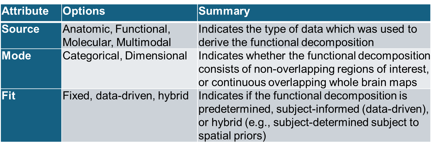
One of the challenges in the field is distinctions between decomposition types are often not made. To enhance clarity, we can categorize functional decompositions in fMRI studies along three primary attributes: source, mode and fit (Table 1). The source attribute distinguishes between anatomic decompositions, derived from structural features such as gyri or cytoarchitectonic areas, and functional decompositions, identified through patterns of coherent neural activity, often captured through resting-state or task-based fMRI, that may not align with structural boundaries. Other types of sources such as generic or molecular information can also be used to derive the atlas.¹⁷ Joint use of multimodal sources, which leverage multiple modalities, e.g., diffusion MRI and fMRI data, can be used to achieve a more comprehensive decomposition.¹⁸ Regarding the mode attribute, decompositions can be categorical, consisting of discrete, binary regions with rigid boundaries (e.g., atlas-based parcellations), or dimensional, i.e., continuous, overlapping representations where network contributions vary across space and time (e.g., ICA,³ gradient mapping, probabilistic atlases). Finally, the fit attribute encompasses 1) predefined decompositions derived from external atlases (i.e., a fixed atlas applied directly to individual data), 2) data-driven decompositions derived directly from the data without prior constraints, creating study specific parcellations from scratch, and 3) hybrid or semi-blind approaches that incorporate spatial priors that are updated or refined based on individual data using data-driven processes (e.g., spatially constrained ICA^5,19). This framework highlights the contrast between traditional categorical, anatomic, predefined approaches and modern dimensional, functional, data-driven decompositions, while also accommodating hybrid methods that flexibly integrate prior information with data-adaptive processes.

Table 1.Attributes of functional decompositions

Provides a way to describe the specific type of functional decomposition that was used, each having its own strengths and limitations.

Most atlas-based approaches, such as the automated anatomic labelling atlas,²⁰ are anatomically derived, categorical, and predefined. Some atlases have multiple options included (e.g., the functional Yeo 17 network²¹ and the multimodal Brainnetome¹ atlases are dimensional but are most often used as categorical and are predefined. The Glasser²² atlas is also multimodal, categorical, and predefined. The NeuroMark approach⁵ is functionally defined, dimensional, and data-driven. In the next section I expand on the use of hybrid models, which start from an atlas or spatial priors and update the maps based on a given subject’s data, highlighting the NeuroMark pipeline. One might also consider extending this further (e.g., a ‘metric’ or ‘method’ attribute might characterize what optimization was used to derive the atlas such as least squares or maximal spatial independence). For now, I limit it to three to keep it simpler.

Hybrid models for functional decomposition

In my opinion, the use of hybrid models for functional decomposition is particularly important for three reasons. First, individual variability can be quite high, and fixed atlases do not capture this variability well. Function connectivity approaches using fixed atlases may be grouping together voxels that have very different temporal coherence or similarity. And secondly, spatial dynamics approaches can benefit from hybrid models, by allowing brain networks to shrink, grow, or otherwise change shape over time, thus providing a more accurate way to capture what I’ll call a ‘functional unit’ for a given network and timepoint. And thirdly, the use of a hybrid approach allows the decomposition to capture individual variability, while also regularizing the results to stabilize the solution.²³ This is also important as issues of reproducibility and generalizability remain pressing. Many biomarkers initially showing promise in controlled studies failed to replicate in independent samples due to methodological heterogeneity or demographic variability.²⁴ More studies focused on cross-study comparison and lifespan research are needed.

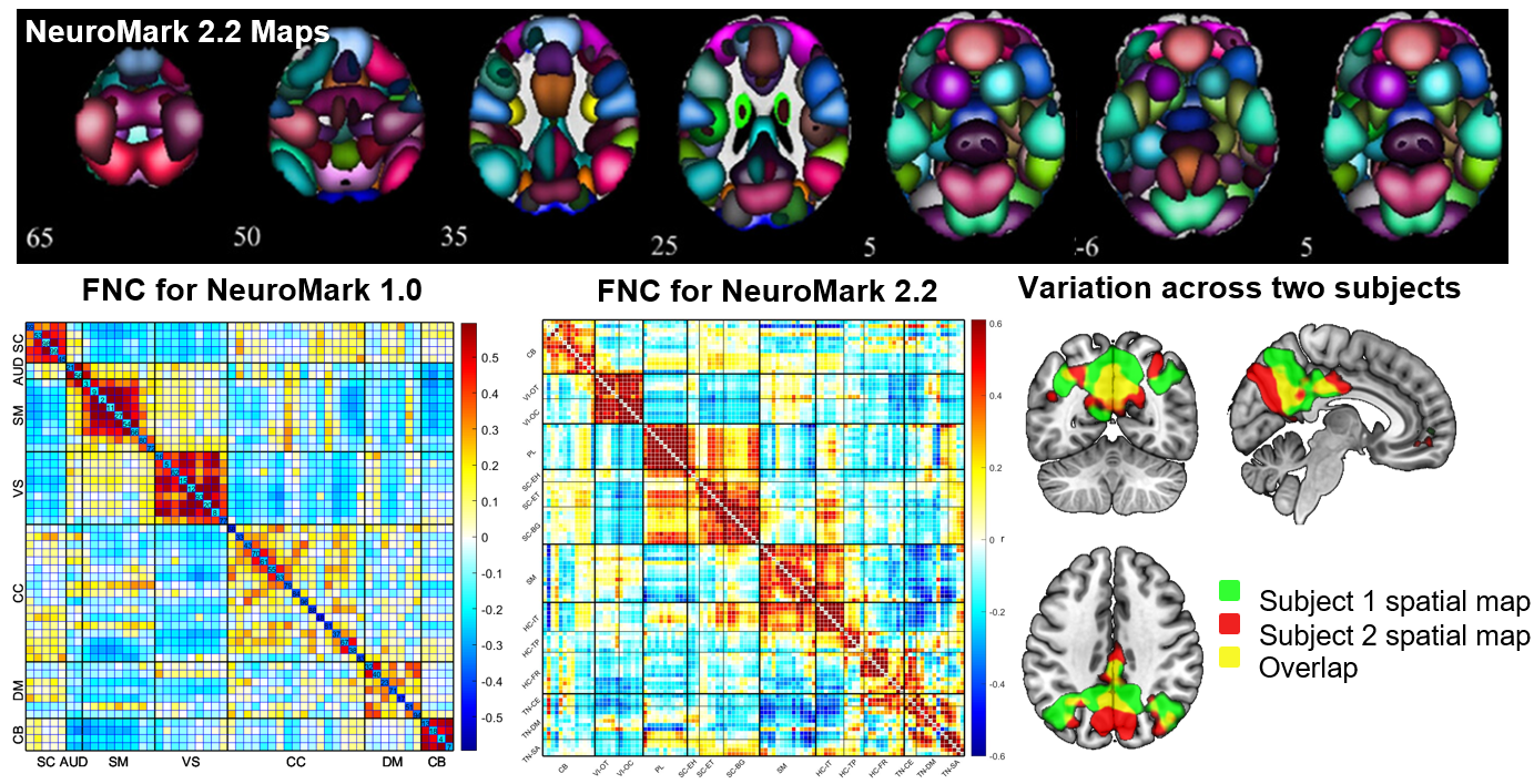
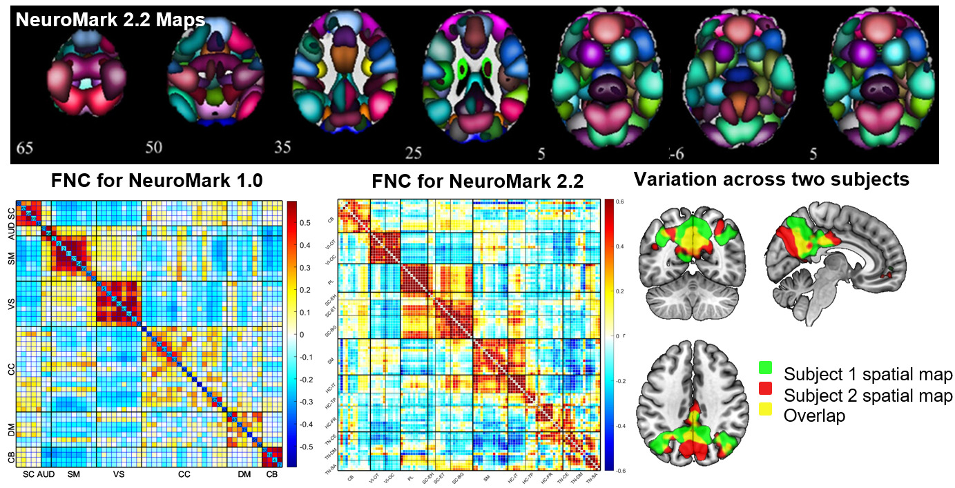
Addressing this requires enhanced standardization in data processing and analysis methods, something we have actively promoted through initiatives like NeuroMark.⁵ In the NeuroMark approach, we use a template initially derived via running blind ICA on multiple large data sets to identify a replicable set of components. These are then used as spatial priors in a single-subject spatially constrained ICA analysis.^19,25 This allows us to estimate subject specific maps and timecourses, while also maintaining the correspondence and ordering of the components between individuals. It also allows us to fully automate the ICA pipeline, while fully leveraging the higher order statistics by computing individual subject spatially informed ICA. Our first NeuroMark template NeuroMark-fMRI-1.0⁵ contains 53 components and has been used in dozens of studies to date. We have also introduced several age-specific NeuroMark templates as well as extending the approach to structural MRI and diffusion MRI data¹³ (all templates available in the GIFT toolbox http://trendscenter.org/‌software/‌gift and at http://trendscenter.org/‌data). We also introduced a multi-scale lifespan atlas which leverages almost 80,000 subjects across a wide range of subject characteristics.¹⁴ This is currently released as NeuroMark 2.2²⁶. Figure 1 (top) shows the coverage for the multi-scale atlas (NeuroMark 2.2) as well as an example of the functional network connectivity (FNC) represented as the cross-correlation between the timecourses within the reference data Figure 1 (bottom middle). Figure 1 (bottom left) shows an example of the FNC for the NeuroMark 1.0 template for comparison. And finally, Figure 1 (bottom right) shows how this hybrid approach captures subject-specific variation within one network for two subjects (green and red are subject specific, yellow is overlap).²⁶ The ability to capture variation between individuals while also providing network-level correspondence highlights the flexibility of an approach that blends the strengths of predetermined and data-driven approaches.

Figure 1.NeuroMark 1.0 and 2.2 templates

NeuroMark 2.2 spatial maps (top), NeuroMark 1.0 (bottom left) and NeuroMark 2.2 (bottom middle) functional network connectivity, and (bottom right) variability among two subjects in one of the NeuroMark 2.2 networks, showing the ability of the hybrid approach to capture individual variation in spatial networks, while also preserving correspondence among subject.

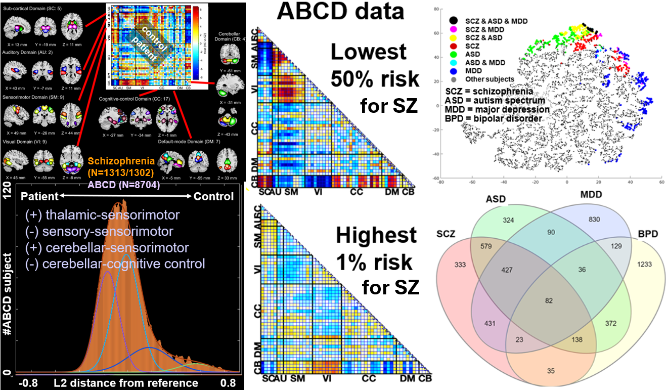
Computing risk scores for neuropsychiatric disorders that can also capture individual variability is of great interest.^27–29 As one example of this approach, I highlight work from 2024 using the NeuroMark framework to develop a brainwide risk score (BRS).³⁰ In this case we generated individualized NeuroMark 1.0 output for approximately 14,000 datasets including clinical datasets from four disorders including schizophrenia (SZ), autism spectrum disorder (ASD), major depression (MDD), and bipolar disorder (BPD), as well as controls, and also for over 8,000 adolescents between the ages of 9-11 within the ABCD dataset baseline cohort. Following preprocessing and quality control, we computed FNC matrices for all individuals and generate clinical reference patterns for each disorder. We then compared individuals in the ABCD dataset to these references using a distance metric and then computed the difference as a brainwide risk score (BRS). Figure 2 (top left) shows the reference pattern for controls and individuals with schizophrenia, along with the NeuroMark spatial maps. Figure 2 (bottom left) shows the histogram of BRS within the ABCD study. Interestingly, results show a skewed relationship. The control-like patterns are strongly represented in over 50% of the ABCD cohort Figure 2 (top middle) whereas the patient-like patterns are only visible in the upper 1% of the cohort, Figure 2 (bottom middle). This is notable as it is consistent with the prevalence of schizophrenia.³¹ The BRSs in these individuals also showed a significant correlation to the prodromal risk score. Since the score is computed separately for each of the four disorders, we can visualize the relationship between the individuals in the upper 5% of risk, Figure 2 (top right) and also the degree to which an individual falls within the upper 5% on each of these histograms, Figure 2 (bottom right). This provides a powerful example of how hybrid approaches can capture dimensional relationships between brain patterns and mental illness reference. It also blends together categorical approaches (reference creation) with a dimensional perspective (similarity) to risk or resilience. It is also worth a brief comment on sample size. While large sample sizes clearly help with generalization, especially in the case of small effects, it is not a requirement; most of the approaches we discuss in this paper are also applicable for small N studies. While the specific context is relevant, to give two examples, generating a new NeuroMark template can greatly benefit from showing robustness and replicability, but once a given template is created, it can be used on an individual subject in a case study, a small N comparison, a pre-post treatment study, or a large N population neuroscience study as we have shown for the ABCD data. However, as is the case with most work, replication is a hallmark of science, and the further one can show that the results will consistently replicate the better. More complex models, e.g., moving to approaches which couple independence with more complex neural network models, will also allow us to accommodate nonlinear relationships (see Figure 4) and incorporate brain network estimation within a powerful ‘end-to-end’ model framework, however the sample sizes required for consistent replication will likely be somewhat larger in these cases.

Figure 2.Brainwide risk score (BRS) analysis using the NeuroMark pipeline.

(Top left) spatial maps and patient/control references, (bottom right) histogram of BRS for ABCD individuals, (top middle) average FNCs for ABCD individuals in the lowest 50% of risk, (bottom middle) average FNCs for ABCD individuals in the upper 1% of risk, (top right) visualization of individual in the upper 5% of risk for each disorder, and (bottom right) Venn diagram showing how many individuals fell into the upper 5% risk for each of the disorders.

Expressive visualization of neuroimaging data

As neuroimaging models grow increasingly complex, the demand for tools that facilitate understanding and discovery has expanded.³² While this is not a new problem for the field, as neuroimaging has always had to focus extensively on ways to visualize and promote understand spatiotemporal data,³³ it has become even more important due to the proliferation of deep learning models which suffer from a “black box” nature, often with millions of parameters and highly nonlinear.³⁴ Although these models excel at prediction, it can be challenging to connect the resulting predictions to meaningful and understandable aspects of the data. This has led to the proliferation of terms such as interpretability, explainability, explainable AI, transparency, and trustworthiness, each touching on different aspects of improving our understanding of a given model.³⁵

Interpretability, explainability, and what we call expressive visualization (EV) are related but distinct concepts, particularly when it comes to AI, machine learning, and complex data analysis. We define interpretability as the degree to which a human can understand the cause-and-effect relationships within a model or system. That is, the focus is on understanding the model’s internal mechanics in a way that makes sense to a human and provides information on how input features relate to outputs. We define explainability as the broader concept of providing understandable descriptions or justifications for model predictions, even when the model itself is complex or opaque (black box). That is, a focus on creating mechanisms or approximations that help a user understand what the model is doing. Explainability tries to provide insights into model predictions without necessarily understanding the internal structure. Complementary to interpretability and explainability is our concept of EV, which emphasizes the importance of providing a rich graphical representation of neuroimaging data or model outputs to reveal the underlying relationships, or structures in the data.

NeuroAI approaches often focus on methods designed to explain model predictions through techniques such as feature importance mapping, saliency analysis, or attention mechanisms.^36–38 However, these methods, while useful for validating predictions and ensuring accountability, are not ideally suited for the discovery of new neural phenomena or emergent properties within large-scale neural systems. One of the ironies here is that, due to the larger parameter space, deep learning provides the opportunity for even richer visualizations than what are available from simpler modeling approaches.

Our emphasis on EV is a call to build rich, multidimensional, and dynamic visual representations that more fully harness the underlying complexity of NeuroAI models. EV is a call to go beyond conventional visualization techniques in order to emphasize the creative and systematic construction of visuals that actively reveal novel structures, patterns, and relationships within neural network representations. EV emphasizes creating visual representations that are not only illustrative but also capable of generating novel scientific insights by exposing patterns, dynamics, and structures that are otherwise obscured by high-dimensional or abstract representations. These would ideally include representation of the spatiotemporal aspects of the original brain data, as well as latent constructs such as state-spaces or gradients. For example, the spatiotemporal nature of brain networks–reflected in metrics such as state-space information, time-varying connectivity, network convergence indices, spatial maps, or latent space trajectories–requires approaches that are sensitive to space and time and possibly temporally evolving structures. Visualizations that capture multiple levels of the results at higher resolutions can provide much more depth to the results (e.g., incorporating decompositions as mentioned earlier can go beyond a single map or include results in the input data resolution or higher rather than a fuzzy attention map). These types of visualization are available to any analysis but often not implemented.

The motivation for EV stems from the realization that traditional interpretability frameworks are insufficient for the level of complexity inherent in contemporary NeuroAI models. Neural networks applied to neuroimaging are characterized by vast numbers of parameters, nonlinear relationships, and temporally evolving dynamics that resist explanation through simple attribution scores or static plots. Instead, what is required is a deliberate effort to build visualization frameworks that are sensitive to these complexities and designed to uncover new insights rather than merely confirm existing hypotheses. EV also facilitates integration of data exploration, statistical rigor, and hypothesis generation. There is some relationship to the concept of explorable explanations, which are visual tools for providing intuition into a concept or a dataset,^39,40 but here we are mainly focused on improving the visualization output for NeuroAI applications. Rather than constraining visualization to the final stages of model interpretation, EV treats the design of visual tools as a core component of the modeling process. This paradigm shift allows researchers to iteratively refine their models and visualizations in tandem, creating a feedback loop that drives discovery.

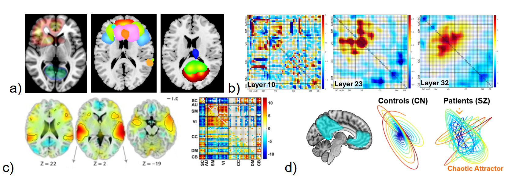
There are many ways to produce rich visualizations from neuroimaging models. Figure 3 shows a few simple examples including salience or attention maps (which by themselves are arguably often blurry and of limited value). There may also be additional value in further decomposing individual subject salience/relevant/attention maps, e.g. via a constrained ICA model to provide “source-based saliency”⁴¹ (Figure 3a). Visualization of multiple layers of a deep residual network highlighting patient versus control differences, or further decompositions of these maps can also provide useful insights into the model (Figure 3b). In addition, we encourage the use of transparent visualization of regions below a statistical threshold^33,42 (Figure 3c). Visualization of the functional decomposition linked to a given dynamical systems approach can go beyond a 2D state space plot, (Figure 3d) shows evidence of chaotic attractors in patients with schizophrenia linked to multiple default mode network nodes extracted via ICA. The EV approach is essentially focused on designing a model with visualization in mind. While this may seem straightforward, it is widely used in NeuroAI. NeuroAI models as represented in research papers tend to have less visualization when they should have more. This is in part evidenced by evaluating NeuroAI papers in recent conferences (e.g., NeurIPS) which show approximately 50% of the papers do not have any or minimal spatiotemporal visualization included in the paper. NeuroAI papers tend to have a larger focus on prediction benchmarks or (in a smaller number of cases) visualization of latent factors, but often much less visualization within the native brain space. As these models advance, it is critical that we enhance our ability to visualize the results while including both spatial and temporal aspects.

Figure 3.Example visualizations of neuroimaging models

(a; left) Salience maps for analysis of ABCD data predicting males vesus females from gray matter maps with over 97% accuracy (increasing with age) F>M (orange) and M>F (blue).⁴³ (a; middle) source-based saliency maps for F>M, (a; right) source-based salience maps for M>F. (b), FNC Control - Patient differences in layer 10, 23, and 32 of a neural network highlighting different levels of granularity for a convolutional neural network model yielding an accuracy of 92.8% in predicting individuals with schizophrenia versus controls,⁴⁴ (c; left) transparent thresholding of spatial maps,^33,42 (c; right) upper/lower triangle with thresholded and unthresholded FNC, (d) visualization of linear dynamical systems + ICA model showing evidence of chaotic attractor in the default mode network.

Independence as a useful tool for studying neuroimaging data

I have spent a considerable portion of my career developing and applying methods that leverage independence–most notably through ICA–to better understand brain function. ICA is widely used in the field and continues to evolve and expand.^45–47 While ICA is perhaps most commonly associated with spatial decomposition of fMRI data, we and others have extended this framework in numerous directions, including temporal ICA^48,49 to isolate distinct time courses, windowed ICA on time-varying functional network connectivity (FNC) matrices to capture dynamic shifts in brain network interactions,⁵⁰ and joint ICA⁵¹ across modalities to identify shared patterns. These approaches all rest on the fundamental assumption that useful insights can be obtained by identifying components that are statistically independent, or as close to independent as possible, across one or more domains (space, time, subject, modality, etc.).

A common critique I’ve encountered is the notion that “it doesn’t make sense to force brain activity into independent parts when we know the brain is highly interactive and coordinated.” This is a reasonable question–one that invites a deeper consideration of what independence really means in the context of data decomposition. Importantly, enforcing independence in the data does not imply a belief that the underlying system (i.e., the brain) itself is comprised of non-interacting parts. Rather, independence serves as a mathematical constraint or organizing principle that enables us to disentangle complex mixtures into more interpretable, constituent signals. These signals may represent distinct sources of variability, modes of processing, or system-level contributions–each of which can be independently modulated even as they participate in larger, interdependent brain functions.

The appeal of ICA lies in its use of higher-order statistics–capturing not just mean and variance (as principal component analysis does), but skewness, kurtosis, and beyond. This allows ICA to separate sources that may overlap spatially or temporally but differ in non-Gaussian structure. It also enables a form of continuous decomposition, in contrast to rigid parcellations or clustering, offering a rich and interpretable visualization of spatial or temporal contributions across the brain. This makes ICA particularly well suited to neuroimaging, where signal mixtures are complex and often reflect subtle but meaningful variations across time, space, and individuals, which are often overlapping with one another.

Moreover, independence is not an endpoint–it is a starting point for deeper analysis. Once independent components are identified, we can study how they interact. For example, dynamic functional network connectivity analyses capture time-varying relationships between ICA-derived components. This allows us to ask how brain systems transiently couple and decouple, fluctuate in synchrony, or evolve during task or rest. So, in essence, ICA does not negate interdependence–it helps reveal it in a more structured and interpretable form. ICA’s utility also extends beyond linear models. The statistical foundation of independence can also be embedded into nonlinear and deep learning frameworks, offering a bridge between classical signal processing and modern AI-driven approaches (e.g., via nonlinear ICA approaches, further optimizing separation of latent factors within a deep learning model, or used to train generative models that can account for additional nonlinearity⁵²; Figure 4). Whether used as a preprocessing tool, a latent representation, or an interpretable model component, the principle of maximizing independence continues to provide value across the evolving landscape of neuroimaging analysis.

Figure 4.Example of the use of a conditional denoising diffusion model, trained on NeuroMark ICA components which can be used to generate single-subject spatial maps for training or individual prediction purposes while also accounting for additional nonlinear effects.⁵²

Dynamic connectivity: Continuously evolving space, connectivity, and states

We continue to see dramatic growth in approaches and applications of time-varying connectivity of fMRI data.^53–55 As the field has matured, there is consistent evidence that time-resolved information is more informative than focusing on static maps alone, both in terms of capturing distinct properties of an individual, and in terms of predictive accuracy (e.g., predicting diagnosis or progression). Evidence increasingly supports the superior sensitivity and clinical utility of dynamic approaches, reinforcing the benefits of temporal modeling.^56,57 While recent work has debated how best to characterize the degree to which various aspects of arousal, global signal, cognition, diagnoses, age, or other factors may contribute to the signal,^58,59 it is clear we are still only scratching the surface of the potential for leveraging brain dynamics. In this context, the brain is a spatiotemporal organ, and as such models should focus on more fully leveraging this information. Here, I call attention to work focused on tapping into the richness of evolving systems of voxels or connectivity patterns in order to more fully capture the dynamic information available in the data. As a brief history, initial whole brain connectivity work focused on estimating static patterns.⁶⁰ This then evolved into estimating transient states of connectivity,⁶¹ followed by models that can capture overlapping states,⁶² and more recently, exponential growth of many different approaches and applications.^53–55 More recently, models have begun to focus on characterizing the continuous evolution of multiple spatial or connectivity patterns (i.e., evolving states).

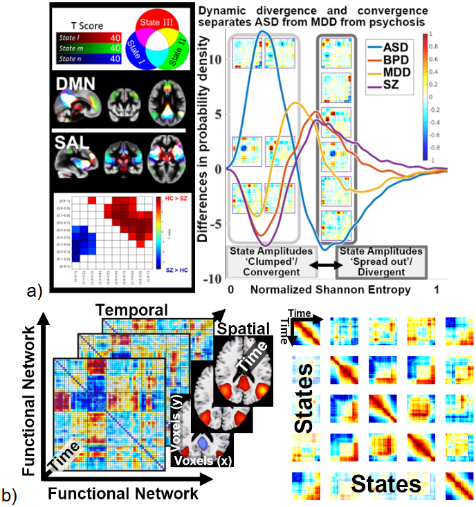
Spatially dynamic approaches (i.e., transiently occurring spatial networks), as opposed to temporal dynamics (i.e., transiently occurring functional connectivity patterns between networks) have grown over the years.^63,64 Figure 5a (left) shows examples of three spatial dynamic states^65,66 which overlap with one another transiently (white regions) and show sensitivity to diagnostic condition. Building on this, we can move beyond a focus on individual non-overlapping states to a more comprehensive summary of the tapestry of continuously evolving and overlapping changes. For example, Figure 5a (right) shows results where windowed FNC matrices were decomposed via ICA, resulting in 15 continuous or fuzzy timecourses, one for each state. We then perform a distributional analysis of the timecourses, that is at each timepoint we compute either a distance between amplitudes or a measure like Shannon entropy to evaluate the degree to which the amplitudes of the states tend to be more ‘clumped’ or more evenly spread out. This measure appears to be remarkably sensitive to neuropsychiatric illness, in particular, it well separates autism spectrum disorder (ASD; blue), major depression (MDD; yellow), and psychosis disorders such as bipolar disorder (BPD; orange) and schizophrenia (SZ; purple).

The second row of figures show examples of evolving states. This can be estimated by applying constrained ICA (e.g., NeuroMark) over time on short windows of data, called dynamic ICA.^50,64 Using this approach we can generate time-varying spatial networks as well as time varying FNC matrices (Figure 5b; left). We can also combine this with the estimation of connectivity states by using a second dynamic ICA to estimate connectivity states, followed by a reference informed ICA to estimate evolving connectivity states.⁵⁰ This provides a wealth of information. A visual example of the richness of this approach is shown in (Figure 5b; right) which shows, for one subject, the similarity of the evolving state patterns to one another. Each square shows the window-by-window similarity between a pair of states. This provides a visual summary of the rich temporal information contained within each of these evolving states, which can be further summarized for characterizing the properties of individuals and groups.

Figure 5.(Top left) spatial dynamic states, showing regions that have higher transient overlap between states (white) versus those that are dominated by just one state (red/blue/green) regions. (Top right) distributional comparison of the amplitudes of 15 states estimated via connectivity ICA show remarkable differences in regions where states amplitude tend to either be clumped together/convergent or spread out/divergent. (Bottom left) evolving FNC state and evolving spatial brain network (we have multiple evolving FNC states and multiple spatial networks; not shown). (Bottom right) chronnectogram characterizes the complex interactions occurring between evolving FNC states within one subject.

Symmetric and dynamic multimodal fusion

• Xue, Y., Li, X., & Zhao, J. (2024). Dynamic multimodal fusion for robust emotion recognition. In Proceedings of the IEEE/CVF Conference on Computer Vision and Pattern Recognition Workshops (CVPRW). https://openaccess.thecvf.com/content/CVPR2023W/MULA/papers/Xue_Dynamic_Multimodal_Fusion_CVPRW_2023_paper.pdf​:contentReference[oaicite:8]{index=8}

Another major focus of my career is on multimodal data fusion. While there are many studies which perform multimodal analysis, there are fewer focused on what is called symmetric fusion, that is joint decomposition of multiple modalities. This is in contrast to asymmetric fusion which involves using one modality to constrain another. Asymmetric fusion is in wide use in the field, e.g. fMRI constrained EEG, diffusion constrained functional connectivity,⁶⁷ or anatomic constrained brain function.⁶⁸

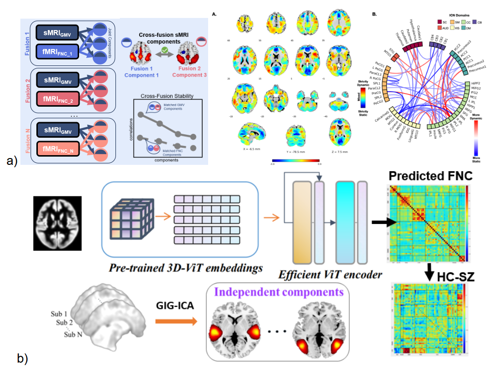
In this section I highlight two recent developments in the field. The first is a new framework called ‘dynamic fusion’ which combines the concepts of symmetric fusion of a pair of modalities within a dynamically defined joint model. While dynamic fusion has been used in other areas such as linking audio and video,⁶⁹ such work tends to focus on the performance rather than the dynamics of the fusion parameters themselves.⁷⁰ However, studying the degree to which fusion of static with dynamic data varies with time represents an important opportunity to study multimodal links in neuroimaging. An initial way to do this is to perform multiple fusions where we might have a static modality, like diffusion or gray matter fused with different functional data^71,72 (Figure 6; top left). This allows us to identify ‘dynamically informed’ structural maps that are more (dynamic) or less (static) sensitive to the time-resolved FNC fusion process. More specifically, we advocate for the creation of structural features (i.e., basis sets/latent representations) in a way that is informed by the dynamically changing functional contexts that individuals oscillate through during a functional scan.

Consider, as an intuitive example, a swinging pendulum system. The system has finite set of physical properties that are unchanging during the observation period (akin to the structural properties of the brain that are unchanging during the course of an MRI scan); however, depending on the functional aspect of interest in the model (e.g., oscillatory motion or energy dissipation), different physical (i.e. “structural”) aspects of the system become salient (e.g., angular position, angular velocity and pendulum length for oscillatory motion, and velocity, surface area, coefficient of drag and friction at pivot for energy dissipation), and thus different structural basis sets are defined for the same system. In the same way, our dynamic fusion approach derives multiple structural basis sets for the same physical brain system that are each best suited to describe the different functional “states” considered across time. In other words, what we derive are temporally evolving patterns of structure-function coupling, rather than short-scale changes in physical brain structure itself. The initial work in this space is quite promising, suggesting both enhanced sensitivity to clinical groups, as well as capturing otherwise hidden relationships which follow along the unimodal to transmodal cortical areas (Figure 6; top right). We have also extended this concept to study imaging genomics links⁷³ as well as links between structure and functional connectivity.⁷⁴

While multimodal methods consistently outperform individual modalities, their complexity and resource demands raise questions about scalability and feasibility. This highlights the need for practical methods that maintain accuracy while being widely implementable. A challenge that often arises is the need for a requirement for multiple modalities to be collected on all individuals in a given analysis, a requirement that typically results in smaller sample sizes than the corresponding unimodal analyses. One aspect that can help with this is the use of generative models. This can provide additional data for training of models, but also provides a way to synthesize data in the case where a given modality might be missing (Figure 6; bottom⁷⁵).

Figure 6.a) A dynamic fusion model incorporates multiple time-resolved symmetric data fusion decompositions (top left) including a static modality (e.g., gray matter) and a dynamic modality (e.g., dynamic FNC), following by evaluation of the similarity of the decomposition of the static modality to identify components which are more or less impacted by dynamicity. Interestingly, structural gray matter dynamic behavior also appears to approximately follow a gradient along unimodal (red) versus heteromodal (blue) cortices (right). (Bottom) generative NeuroAI models can be used to synthesize multimodal data (in this case we show an example of generating functional data from structural data).⁷⁶ This solves a major challenge with multimodal analysis which often have much smaller samples due to missing modalities.

Conclusion

A guiding principle of my career–staying close to the data–has consistently driven innovation in the development of neuroimaging biomarkers. By grounding analysis in empirical signals while thoughtfully integrating model-based frameworks, we have gained deeper insights into the complexities of brain function and dysfunction. Evolving research over the last year brought significant advancements, unexpected findings, and important debates, but also highlighted critical opportunities for refinement and progress. Moving forward, I believe our field will benefit most from a continued commitment to methodological rigor, transparency, interdisciplinary collaboration, and open scientific dialogue. While I have highlighted my own views and approaches in this manuscript, without direct experimental comparison to alternative methods (see our primary papers for some of these comparisons) I also want to affirm my strong belief in the strengths of a pluralistic analytic approach. There are many available methods to choose from, each with their own advantages and limitations. While multiverse studies often focus on common finding across methods, I think it is just as important to highlight where methods differ, as this can in some cases is tied to a specific methodological strength and may provide critical clues about how the brain works. My own journey affirms that remaining anchored in the data, persistently questioning assumptions, and bridging exploratory analyses with principled modeling are essential for realizing the next wave of discoveries in neuroscience–and for translating those discoveries into meaningful clinical impact.

Acknowledgements

I want to thank the students in my lab who performed analysis that led to some of the included figures, including Lord Wiafe, Najme Soleimani, Kyle Jensen, and Yuda Bi, and the core work done by Armin Iraji, Marlena Duda, Jiayu Chen, Meenu Ajith, Zening Fu and many more folks at TReNDS.

Funding Sources

This work was supported by National Institutes of Health grant numbers R01EB006841, R01MH118695, R01MH117107, and RF1AG063153 and NSF grant 2112455.

Conflicts of Interest

The author declares no competing interests.