Canonical time-series features for characterizing biologically informative dynamical patterns in fMRI

Introduction

The study of how systems evolve over time is ubiquitous across the sciences, with contributions to time-series analysis from fields ranging from biomedicine to astrophysics. Recent work has assembled these myriad techniques into a unified library of over 7000 time-series ‘features’—the hctsa feature set^1,2—where each feature encapsulates an interpretable (real-valued) property of a time series. Time-series features quantitatively capture diverse properties from the dynamics of a process, such as how periodic it is, how it distributes its energy across different frequency components, how predictable it is, how nonlinear the dynamics are, and the timescale-scaling of its fluctuations.

In large-scale neural systems, the dynamics of individual brain regions have been shown to vary along a unimodal–transmodal axis,³ vary with structural connectivity strength^4,5 and cortical microstructure,⁶ distinguish between individuals,⁷ characterize sleep states⁸ and anesthesia,⁹ and be disrupted across psychiatric and developmental disorders.^10,11 While many analyses of fMRI time series have focused on estimates of timescales—typically variations on the rate of decay of the autocorrelation function, or low-frequency spectral power—the existence of a large time-series feature library in hctsa allows us to compare a wide range of potential time-series properties. However, hctsa was designed as a comprehensive survey of the interdisciplinary time-series analysis literature and thus contains a large number of highly correlated features.^1,12 For any given problem, or class of problems, we would like to distill the thousands of candidate features in hctsa down to a concise subset of the most informative time-series features that is efficient to compute and reduces the statistical comparison burden of the resulting analyses. Recent work demonstrated one approach to this problem: the thousands of hctsa features were reduced down to a high-performing and representative subset of 22 time-series features, called catch22.¹³ This work defined high-performing features as those with the best performance across a diverse set of 93 time-series classification problems,¹⁴ and then used hierarchical clustering to reduce inter-feature redundancy, yielding a reduced set of 22 features. Feature performance was quantified using a set of 93 time-series classification tasks that span a wide range of general applications, from identifying birds using time series extracted from binary images¹⁵ through to distinguishing types of coffee from their infrared spectra.¹⁶

While catch22 is a high-performing and efficient general-purpose time-series feature set, tailoring features to a specific problem is still needed to optimally characterize the relevant dynamical properties.¹⁷ Previous analyses of fMRI time series have involved two main issues. For studies that hand-select a single feature of interest (like a metric of autocorrelation timescale),^4,5 the large range of alternative features are left untested, leaving open the possibility that alternative statistics could be more informative and interpretable. Applications that have systematically compared the performance across a large feature library, such as hctsa,^{3,6,8,18–20} have involved substantial computational expense and statistical care in dealing with high-dimensional feature spaces (often requiring correction across thousands of features, limiting the power to detect signals in smaller samples). fMRI time series are short, noisy, and—particularly in the resting-state regime where dynamics may be approximated as close to a steady-state—are generally well-suited to being characterized by linear time-series analysis methods.^21,22 However, some prior work has shown that novel time-series methods can reveal new insights into macroscopic brain organization: accurately tracking independent biological gradients in human brains,³ classifying stimulation experiments in mice,^18,19 and distinguishing experienced meditators from controls using resting-state EEG.²⁰

Here we aimed to develop a computationally efficient time-series feature set tailored to capturing informative dynamical patterns in fMRI time series, focusing mainly on the example of mouse fMRI (but later testing on independent datasets from both mouse and human). Successfully building an efficient reduced set of time-series features to characterize fMRI could thus facilitate new research into quantifying local dynamics in neuroimaging, allowing comparisons beyond conventional metrics, without the statistical and computational burden of evaluating thousands of candidate features. To judge the usefulness of different time-series features in this setting, we used data from recent experiments in mice using targeted chemogenetic manipulations of the underlying neural circuits (including excitatory and inhibitory neuronal firing rates) and measuring the fMRI dynamics in response.¹⁸ These labeled data allowed us to score each time-series feature by how well it distinguishes biologically meaningful manipulations to the neural circuits. We introduce improvements to the catch22 pipeline for constructing a reduced set of time-series features from a large feature library (such as hctsa) and use this improved pipeline to extract a set of 16 highly informative time-series features, which we term the catchaMouse16 feature set—producing an efficient and open software package for use by the community. We show that the performance of this set of 16 features in classifying different viral designer receptor exclusively activated by designer drug (DREADD) manipulations approximates that of the full set of $>7000$ hctsa features and, consistent with it capturing biologically informative dynamical information, catchaMouse16 also performs well on unseen tasks involving mouse fMRI.

Methods

Our main aim was to reduce the comprehensive hctsa set of $>7000$ candidate time-series features² down to a subset that displays similarly strong performance in distinguishing fMRI dynamics corresponding to biologically meaningful changes at the circuit-level, assessed using a dataset of chemogenetic manipulations to mouse cortical circuits.¹⁸ In this section, we describe the data and corresponding classification tasks used to score the performance of individual time-series features. We then describe our method for setting the parameters of a feature-reduction pipeline, adapted from Lubba et al.,¹³ using a leave-one-task-out cross-validation approach. Code to reproduce our analysis is available at https://github.com/DynamicsAndNeuralSystems/catchaMouse16_paper_code.

Dataset

Here we consider a set of time-series classification tasks based on distinguishing different chemogenetic manipulations from fMRI time series. We use data described in Markicevic et al.,¹⁸ where full experimental details can be found; key information is summarized here. Note that the original study was carried out in strict accordance with the Swiss Federal Ordinance for Animal Experimentation and approved by Zurich Cantonal Veterinary Office (ZH238/15); no new data were collected in this study. Chemogenetic manipulations were made in the primary somatosensory area (SSp) in the right hemisphere of the mouse isocortex. As well as the control condition (labeled ‘SHAM’ here), three chemogenetic manipulations were performed: (i) activating hM3Dq-DREADD in wild-type mice, which increases overall neural excitability (labeled ‘excitatory’ here); (ii) activating CaMKIIa-hSyn-hM3Dq-DREADD in wild-type mice, which selectively increases the excitability of pyramidal neurons (labeled ‘CAMK’ here); and (iii) activating inhibitory hSyn-dlox-hM4Di-DREADD in PVCre mice, which selectively decreases the excitability of PV interneurons (labeled ‘PVCre’ here).

From this dataset, we constructed twelve classification tasks in total: six based on data from the right-hemisphere SSp (spatial site of the injected DREADD) and six based on data from the contralateral left-hemisphere SSp. In each region, the six classification tasks corresponded to all pairwise combinations of the four labeled classes: ‘SHAM’ (13 fMRI time series), ‘excitatory’ (14), ‘CAMK’ (13), and ‘PVCre’ (19). We labeled each of these twelve tasks in the form region-group1_group2, such that r-SSp-CAMK_PVCre corresponds to the task in which the goal is to distinguish CAMK and PVCre manipulations in the right-hemisphere SSp.

Feature extraction, scoring, and reduction

We used hctsa (v1.03) to extract the full hctsa feature set from all 118 (59 left-hemisphere and 59 right) time series in the dataset. Missing or special-valued outputs that occurred in any of the 12 classification tasks were ignored in subsequent calculations. After filtering, all remaining features were normalized as a $z$-score. A total of $F = 6356$ hctsa features survived filtering across all tasks and were included in the remaining analysis. In each task, every feature was scored according to its balanced classification accuracy using a linear support vector machine (SVM) using the SVM module of scikit-learn.²³ The results were then represented as a task $\times$ feature ($12 \times F$) performance matrix (where each element in the matrix captures the performance of a given feature in a given task).

From the performance results per feature, we aimed to determine a reduced set of features that exhibit strong performance across the set of classification tasks while minimizing inter-feature redundancy, as per Lubba et al.¹³ We follow a similar two-stage approach as Lubba et al.,¹³ first selecting the $\beta$ features with the highest average balanced classification accuracy across the 12 tasks, and then clustering them to reduce redundancy. For this second step, we used hierarchical average linkage clustering, replacing each cluster of highly correlated features with a single representative feature. We defined feature–feature dissimilarity as $1 - |R|$, where $R$ is the Pearson correlation between their performance values across the 12 classification tasks.¹³ In this way, groups of features with similar patterns of classification strengths and weaknesses across classification tasks cluster together (and are therefore considered ‘redundant’ with each other). We cut the resulting dendrogram at a threshold $\gamma$ and represented each cluster as the highest-performing feature in the cluster where possible and, when performance differences were minimal, used scientific judgement when replacing some computationally expensive features with simpler and more interpretable alternatives within a cluster to enhance speed and interpretability. In Lubba et al.,¹³ $\gamma$ was set manually to $\gamma = 0.2$, corresponding to clusters containing features with highly correlated performance $|R| > 0.8$. We used ‘average’ linkage clustering here as we found that it yields superior cross-validated results than the stricter ‘complete’ linkage clustering used previously¹³ (see Fig. S3).

This pipeline for constructing reduced sets of features thus depends on the selection of $\beta$ and $\gamma$. Here we extend the approach of Lubba et al.¹³ by introducing a data-driven approach to select the values of $\beta$ and $\gamma$, using leave-one-task-out cross-validation. In this scheme, for a given setting $(\beta,\gamma)$, a reduced feature set was constructed using data from 11 of the 12 datasets, leaving the left-out dataset as an out-of-sample test. Performance in the left-out dataset was taken to be the 10-fold cross-validation balanced accuracy, using the feature set constructed from the 11 training datasets. The performance of a reduced time-series feature set obtained using given parameters, $(\beta, \gamma)$, was calculated as the average classification performance of that feature set across all 12 left-out tasks. This procedure allowed us to select a value for $\beta$ and $\gamma$ to then use on the full set of 12 datasets to produce a final set of features, catchaMouse16.

Results

Our results are organized as follows. First, we describe our leave-one-task-out method for selecting appropriate parameters of our feature-reduction pipeline and how this yields the catchaMouse16 feature set. We then characterize the composition of this feature set and evaluate its performance relative to the entire hctsa feature set. Finally, we show that catchaMouse16 performs well in independent datasets comprised of mouse and human fMRI time series, in which cortical variations in cell densities are well captured by the variation of catchaMouse16 features of the resting-state fMRI dynamics.

Computing a reduced feature set

In this section, we describe our leave-one-task-out procedure for generating the reduced feature set, catchaMouse16, from the twelve classification tasks derived from Markicevic et al.¹⁸ In first selecting an appropriate value of $\beta$, we note the tradeoff between including too many top features (high $\beta$), resulting in the inclusion of lower-performing features, and including too few features (low $\beta$) which narrows the diversity of potentially complementary high-performing time-series analysis methods. We expected a good value of $\beta$, the number of top features retained prior to clustering, to be similar to that which worked well in the prior study of Lubba et al.,¹³ i.e., $\beta = 100$. Indeed, comparing across values $\beta = 25, 50, 100, 200, 400$, we found that good performance was obtained at $\beta = 100$, with similar performance obtained at higher values of $\beta = 200, 400$ but deteriorated performance at lower $\beta = 25, 50$ (cf. Fig. S1). In preferencing smaller feature sets (low $\beta$), this suggests $\beta = 100$ as an appropriate choice for capturing the diversity of high-performing time-series analysis methods.

To understand how the clustering threshold $\gamma$ affects performance on left-out tasks, we fixed $\beta = 100$ and explored the accuracy on each of the twelve tasks across a set of thresholds $\gamma = 0.05, 0.1, 0.2, 0.3, 0.4, 0.5$. Note that for each left-out dataset, the 11 training datasets are used to select a reduced set of features, and a classification model is then trained and evaluated on the left-out dataset.

Figure 1.A leave-one-task-out procedure allowed us to select a high-performing clustering threshold, $\gamma$.

Results are shown here for the example of clustering the $\beta$ = 100 highest-performing features across the 12 tasks down to a reduced subset, comparing the results of using $\gamma$= 0.05, 0.1, 0.2, 0.3, 0.4, 0.5. A We plot this task $\times$ threshold matrix that shows the results of the leave-one-task-out procedure as a heat map. The number of features used in the model (selected from the other tasks) is annotated to each element, and the balanced accuracy in classifying the left-out-task is shown as color. Left-out tasks (rows) have been sorted by mean balanced accuracy from high (top) to low (bottom). B The distribution of balanced accuracies aggregated across all tasks (i.e., aggregating down columns of the matrix shown in A) is shown as a violin plot for each threshold $\gamma$. Note that the number of retained features decreases with $\gamma$, and varies across left-out tasks, as annotated in A.

Results are shown for all tasks and thresholds in Fig. 1A, showing the number of features selected from the other tasks (numerical annotations) and balanced accuracy on that left-out task (color). We first note that clustering at higher thresholds, $\gamma$, corresponds to larger clusters and thus fewer features in the final feature set, with performance broadly degrading at high thresholds, $\gamma$ (corresponding to fewer features). The trade-off involved in the feature-set reduction problem is thus clearly visible as aiming to produce as high out-of-sample performance while using as few features as possible.

Comparing tasks (rows) of Fig. 1A, we see a range of accuracies across the different tasks: high performance is obtained on some tasks (even with few features), while other tasks display relatively poor performance. The four tasks with the highest classification accuracy in the original analysis by Markicevic et al.¹⁸—r-SSp-Exc_SHAM, l-SSp-CAMK_SHAM, r-SSp-PVCre_SHAM, and r-SSp-CAMK_SHAM—are also the four tasks with highest performance here. High performance on these tasks was mostly maintained across $\gamma$ values; indeed, even at high $\gamma = 0.5$, we see similar classification rates with just a few features (selected from the other 11 tasks). In contrast, tasks like l-SSp-Exc_SHAM and l-SSp-CAMK_PVCre, exhibit a substantial drop in performance when going from a large feature set (low $\gamma$) to a smaller feature set (high $\gamma$).

To select a value for $\gamma$ to apply to the full dataset in constructing catchaMouse16, we examined the distributions of left-out performance, shown in Fig. 1B. The median accuracy across left-out tasks remains approximately constant for $\gamma = 0.05, 0.1, 0.2$ but drops from $\gamma = 0.3, 0.4, 0.5$. This suggests that we can maintain performance while reducing the size of the feature set by selecting $\gamma = 0.2$.

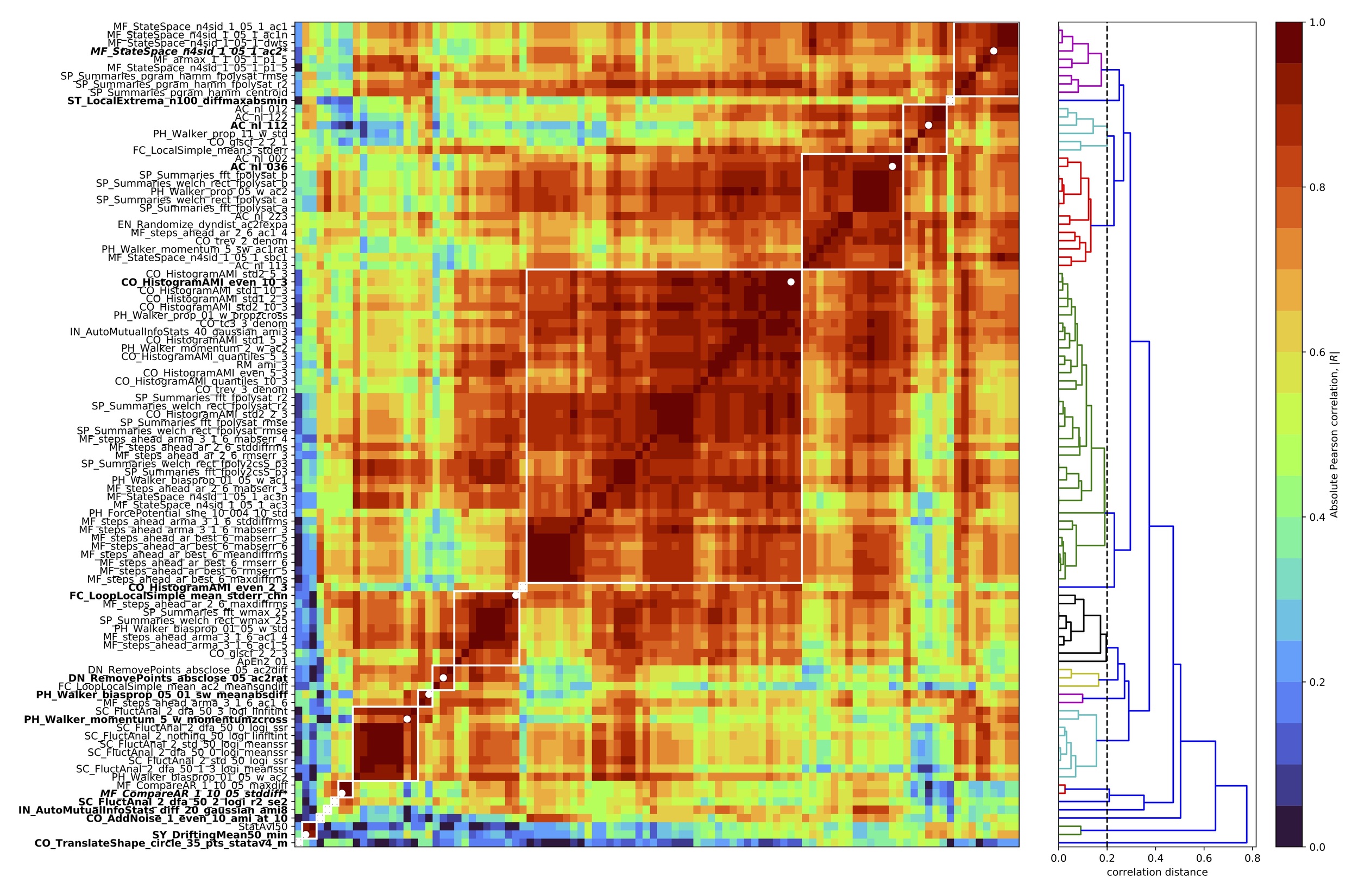
Having selected parameters $\beta = 100$, $\gamma = 0.2$, we applied our feature-reduction pipeline with these settings to the full set of 12 classification problems to compute a reduced time-series feature set. This yielded 16 clusters of high-performing features, shown as an annotated feature–feature correlation matrix in Fig. 2. We then selected a representative feature from each cluster, using scientific judgement to select a high-performing representative that was as simple to interpret and computationally inexpensive as possible, as per Lubba et al.¹³ The resulting set of 16 features is the catchaMouse16 set.

Figure 2.Feature–feature correlation matrix of the 100 top-performing features across the 12 mouse fMRI classification tasks.

A heatmap shows the absolute Pearson correlations between each pair of features, as $|R|$, computed from the variation in performance values across the 12 tasks. Features in the catchaMouse16 feature set are denoted in bold, while the italic features marked with an asterisk denote features which were substituted for similar but easier-to-compute features. The average hierarchical linkage dendrogram used to determine the clusters at a threshold $\gamma$ = 0.2 (annotated) is shown to the right of the heatmap.

The catchaMouse16 feature set

Having determined a reduced set of 16 time-series features, designed to be concentrated in the types of dynamical structures that are most relevant to changes in the underlying neural circuits, we next describe the time-series features in the catchaMouse16 feature set. The features are listed in Table S1, where we have assigned a short name to each feature for ease-of-use. The catchaMouse16 features mainly comprise measures of predictability, such as nonlinear autocorrelations, automutual information estimates, and estimates of long-range scaling of correlation structure.

Three catchaMouse16 features compute different nonlinear time-averages of the $z$-scored time series $x_t$, as: $\langle x_t^2 \,x_{t-3}\, x_{t-6} \rangle_t$ (nonlin_autocorr_036), $\langle x_t^2\, x_{t-3}\, x_{t-5} \rangle_t$ (nonlin_autocorr_035), and $\langle x_t\, x_{t-1}^2\, x_{t-2} \rangle_t$ (nonlin_autocorr_112). Two other features measure nonlinear time-lagged correlations via automutual information: ami3_10bin and ami3_2bin measure the automutual information at a time-lag of 3 samples using a 10-bin (and 2-bin) histogram estimation method, respectively. Another feature, increment_ami8, measures linear time-lagged correlation at a lag of 8 samples, using a linear Gaussian estimator for automutual information.

A range of other catchaMouse16 features capture different aspects of time-series predictability. The noise_titration feature is inspired by the noise titration method of Poon and Barahona,²⁴ which measures the lag-1 automutual information after adding white measurement noise (with a signal-to-noise-ratio of 1) to the time series. And prediction_scale captures the change in prediction error from a mean forecasting method when incorporating increasing durations of prior data into the prediction. The dfa_longscale_fit feature estimates a timescale–fluctuation curve using detrended fluctuation analysis (DFA)²⁵ with quadratic detrending in each window (and returns the standard error in the mean of a robust fit to a long-timescale fluctuation scaling regime). Other more novel features of local shape-like patterns in the time series include the variability of how many time-series points sit inside a circle being translated across the time domain (floating_circle), and two measures of the statistics of a simulated mechanical particle (or ‘walker’) being driven by the time series (walker_crossings and walker_diff).^1,2

Two catchaMouse16 features capture aspects of the stationarity of the signal.¹⁷ First, stationarity_min divides the time series into 50 windows and then measures the minimum windowed mean in any segment divided by the mean variance across windows. And stationarity_floating_circle measures the stationarity across four partitions of the time series (using a quantity called StatAv²⁶) of the statistics of local time-series shapes (number of points sitting inside circles translated across the time series).

Finally, catchaMouse16 contains two measures related to outliers in the time series. outlier_corr computes how the autocorrelation at lag 2 changes after removing 50% of the time-series values closest to the mean. And outlier_asymmetry measures asymmetry in extreme local events by dividing the time series into 100 segments and computing the average difference between the greatest deviation in positive and negative directions.

Together, the catchaMouse16 features aim to provide a concise but multifaceted signature of BOLD dynamics, covering linear and nonlinear correlation structure, scaling behavior, statistics of local shapes, stationarity, and outliers. For broader use, this feature set has been re-coded from the original Matlab into C, and is made available as an open-source package, catchaMouse16, with wrappers for Matlab and Python, available at https://github.com/DynamicsAndNeuralSystems/catchaMouse16.

We analyzed the performance of the catchaMouse16 feature set on the 12 classification tasks from Markicevic et al.¹⁸ As shown in Fig. 3A, the catchaMouse16 features yield similar performance as the full hctsa feature set across the 12 tasks. Further, the feature set performs similarly to the centroids of the feature clusters as outlined in Fig. 2, with the added advantage of being more clearly interpretable and simpler to compute (see supplementary Fig. S2 for details). Although this analysis is ‘in-sample’ in the sense that it is performed on the same dataset on which the catchaMouse16 features were constructed (analyses on independent datasets are presented in the next section), these results indicate that catchaMouse16 can differentiate underlying neural stimulations from non-invasively measured fMRI time series using just 16 features (with similar or greater accuracy as the full hctsa set of $\sim7000$ features).

To characterize the relative computational efficiency of the Matlab implementation of the catchaMouse16 feature set compared to the C-coded version introduced here, we evaluated the feature set on i.i.d. random-number time series of length 900 (repeating the process 2000 times). Results are shown in Fig. 3B, and indicate a $\sim 60\times$ speed-up of the C implementation (and corresponding Matlab mex wrappers) relative to the native Matlab code from hctsa. We find that catchaMouse16 is highly efficient at quantifying dynamical structure in time series, making it suitable for scaling up to large time-series datasets.

Figure 3.The catchaMouse16 feature set maintains high performance with substantial gains in computational efficiency relative to hctsa.

A: Mean 10-fold cross validated balanced classification accuracy of catchaMouse16 (vertical axis) versus hctsa (horizontal axis) across the twelve classification tasks analyzed here. Error bars indicate standard deviations across folds. B: Execution time of the catchaMouse16 feature set in native Matlab code, C code run through Matlab (mex), and in compiled C.

Validation: tracking cell-density variation across brain areas

In this section, we aimed to test the generalizability of catchaMouse16 (which aims to be an efficient and information-concentrated subset of hctsa) on new problems involving fMRI data. Specifically, we aimed to detect statistics of resting-state BOLD dynamics that vary with the relative density of different neuronal types across brain areas (in both mouse and human). In mouse, we focused on pyramidal (excitatory) neurons as well as the three main subtypes of inhibitory interneurons: parvalbumin (PV), vasoactive intestinal peptide (VIP), and somatostatin (SST) expressing interneurons.²⁷ While the densities of all classes of interneurons vary substantially across the cortex,^28,29 the precise roles of interneuron subtypes in shaping macroscopic neural activity remain unclear.^30,31 Identifying time-series features of fMRI dynamics that correlate strongly with the density of interneuron subtypes would be a step toward connecting non-invasive measurements of macroscopic dynamics with the microscopic properties of neuronal circuits. We compared the performance of both hctsa and catchaMouse16 time-series features, reasoning that if the smaller catchaMouse16 feature set can capture the main variation as well as the full hctsa feature set, then this would support it being an information-rich set of informative dynamical properties of fMRI time series.

We used a dataset of resting-state fMRI recordings from 38 regions of the isocortex in the right hemisphere of 100 mice (each of length $T = 900$ samples)^5,32,33 (parcellated according to the Allen Mouse Brain atlas³⁴). For each feature-extraction pipeline (either hctsa v1.03, 7664 time-series features; or catchaMouse16, 16 time-series features), we extracted features from each of the 3800 BOLD time series. We then agglomerated the result for each feature and each brain region by calculating a mean value across all 100 mice (excluding any missing or NaN values). In the case of the hctsa feature set, this yielded a $169 \times 7664$ averaged matrix (region $\times$ features).

In mouse, we compared the spatial variation of each time-series feature (across brain areas) to data on their relative cellular composition obtained from two sources: (i) densities of PV, VIP, and SST interneurons, obtained by cell counting²⁸; and (ii) densities of excitatory and inhibitory populations, estimated from an algorithmic reconstruction of neuronal soma.³⁵ We combined these two sources of cell-density measurements to produce a table of PV, SST, VIP, and inhibitory cell densities for each region in the mouse brain. We repeated the same approach on human resting-state fMRI data obtained from 100 participants in the Human Connectome Project.³⁶ These data, comprising processed and parcellated time series for $180$ left-hemisphere brain regions using the Glasser parcellation,³⁷ were taken from Fallon et al.⁴). As a proxy for PV interneuron density in the human cortex, we used expression of the PVALB gene, taken from Arnatkeviciūtė, Fulcher, and Fornito.³⁸ We chose to focus just on the PVALB gene in humans, as it is the most reliable marker for the corresponding interneuron type (PV) in mouse (as found here, cf. Fig. 5, and in prior work³⁹), whereas the correspondence between genetic markers for SSP and VIP and their ground-truth densities is less clear.³⁹ In both the mouse and human datasets, we quantified the relationship between neuron densities and statistical features of BOLD time series across brain areas using the Spearman correlation, $\rho$. We assessed corrected statistical significance using the Bonferroni–Holm method,⁴⁰ noting that such correction is considerably more stringent for the hctsa feature set (where thousands of features are tested) than the catchaMouse16 feature set (where only 16 features are tested).

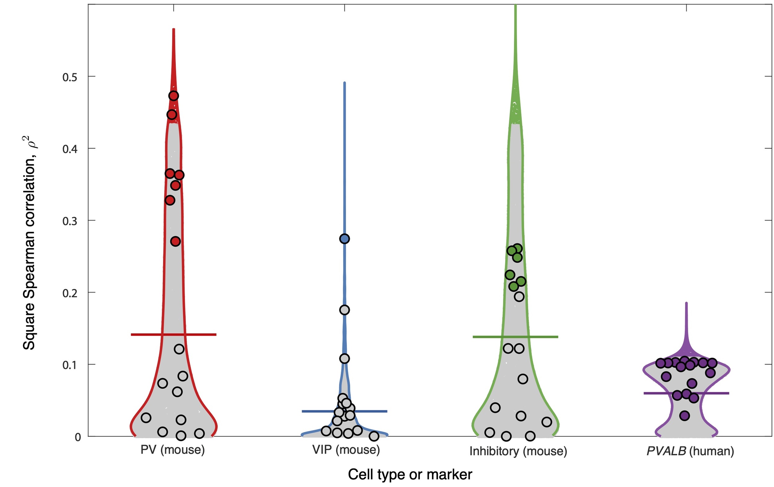
We first analyzed the relationship between fMRI time-series features and cell densities in the 38 regions of the mouse isocortex and PVALB expression in the 180 regions of the human cortex. Of the six cell-type density associations tested, four exhibited a significant correlation with at least one time-series feature: PV, VIP, and inhibitory cells in mouse, and PVALB expression in human. In the other two cases, excitatory cell density and SST cell density in mouse, there were no significant correlations to any time-series features of BOLD dynamics (in neither hctsa nor catchaMouse16). Figure 4 shows the distributions of squared correlations, $\rho^2$, across all BOLD time-series features in catchaMouse16 and hctsa for the four settings in which there was at least one feature with a significant correlation. The distributions of hctsa features are shown as violin plots, with catchaMouse16 features overlayed as circular markers and features with significant correlations ($p_\mathrm{corr} < 0.05$) highlighted in color. For hctsa, we observed significant correlations between individual time-series features of resting-state BOLD dynamics and mouse PV cell density (240 significant features, up to $\rho = 0.75, p < 10^{-3}$), mouse VIP cell density (1 significant feature: lag-21 autocorrelation, $\rho = -0.70$, $p = 7 \times 10^{-3}$), overall mouse inhibitory cell density (249 significant features, up to $\rho = 0.78 , p < 10^{-4}$), and human PVALB expression (273 significant features, up to $\rho = 0.32$, $p = 2 \times 10^{-4}$). A complete list of correlations and $p$-values for each hctsa feature and each cell type is given in Supplementary files PV_7664.csv, VIP_7764.csv, and Inhibitory_7764.csv, and, for human, Pvalb_7764.csv.

Using the catchaMouse16 feature set yielded a significant relationship in all settings that hctsa did. Furthermore, the proportion of catchaMouse16 features that were significantly correlated with each anatomical measurement was far greater than for hctsa, with the top-performing catchaMouse16 feature mostly yielding a similarly strong correlation to the top hctsa feature (in all cases except the overall inhibitory density analysis). The strongest associations to catchaMouse16 features also varied in interesting ways between the cell types. For example, the catchaMouse16 feature with the strongest correlation to the spatial variation in PV cell density was nonlin_autocorr_036 ($\rho = -0.69, p_\mathrm{corr} < 10^{-4}$, cf. Table S2 for all results), with similar types of self-correlation-based time-series features performing well at tracking total inhibitory cell density, including nonlin_autocorr_036 ($\rho = 0.5$, $p_\mathrm{corr} = 0.02$), although with weaker $\rho^2$ than the top hctsa features. By contrast, VIP density exhibited the strongest correlation to dfa_longscale_fit ($\rho = 0.52$, $p_\mathrm{corr} = 0.01$, cf. Table S3 for all results). Overall, the features with the highest $\rho$ with respect to the inhibitory cell density had lower $\rho$ with respect to the VIP cell density; for example, noise_titration has $\rho = -0.51$ ($p_\mathrm{corr} = 0.02$) for inhibitory cells, and $\rho = 0.086$ ($p_\mathrm{corr} = 1$) for VIP cells (cf. Table S3 and Table S4). In the human cortical PVALB analysis, all catchaMouse16 features exhibited a significant correlation (with the strongest correlations being with features capturing nonlinear autocorrelations, like nonlin_autocorr_036, $\rho = 0.32$, $p < 10^{-3}$, and automutual information, like ami3_2bin, $\rho = 0.32$, $p < 10^{-3}$, cf. Table S5). These results suggest that catchaMouse16 can act as a compact and computationally efficient distillation of the time-series analysis literature that is suitable for capturing biologically relevant properties of fMRI dynamics.

Figure 4.catchaMouse16 efficiently captures dynamical properties of mouse and human resting-state BOLD time series that are informative of regional variations in interneuron density across the cortex.

The distribution of squared Spearman correlation coefficients, $\rho^2$, between hctsa feature values of BOLD time series and estimated interneuron cortical cell densities are shown as a violin plot for each cell type or marker.
Gray points represent features with $p_\mathrm{corr} \geq 0.05$; colored points represent features with $p_\mathrm{corr} < 0.05$.
The mean correlation across hctsa features is indicated by a horizontal line.
The 16 catchaMouse16 features are annotated as larger circles, shown as filled gray circles ($p_\mathrm{corr} \geq 0.05$) or filled colored circles ($p_\mathrm{corr} < 0.05$).
As annotated, the PV, VIP, and inhibitory cell densities correspond to mouse data, whereas the PVALB marker is from human data.

Figure 5.catchaMouse16 is enriched in features that are significantly correlated to the cortical variation of interneuron cell densities in all cytoarchitectural layers of the mouse cortex.

The number of features with significant correlations to regional neuronal densities ($p_\mathrm{corr} < 0.05$, Bonferroni–Holm corrected across all features within a given feature set), is shown in a heatmap for both hctsa (A) and catchaMouse16 (B).
Each annotated number corresponds to the maximum Spearman’s correlation for a combination of layer and cell type.
Rows 1-5 were calculated using cell-type densities in one of layers $1-6$ in the mouse isocortex, while row 6 uses densities across all layers in each isocortical region.
Note the color axis of A spans approximately 10% of the hctsa features, whereas the color axis of B spans most of the catchaMouse16 features.

Layer-specific study

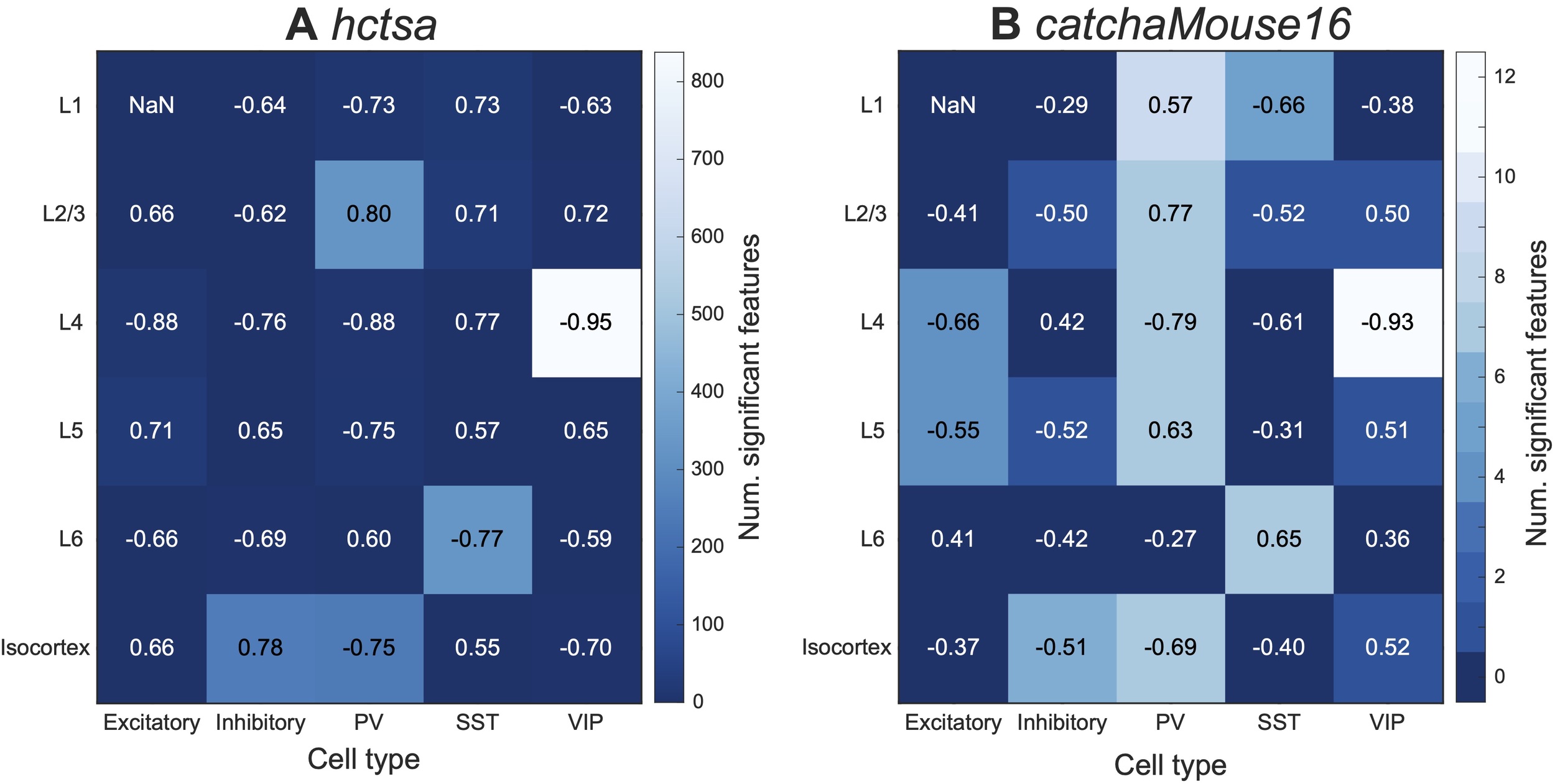
As a final study of the statistical relationship between interneuron densities and fMRI dynamics in mouse cortex, we broadened our scope to compare the catchaMouse16 time-series features of the regional BOLD signal with layer-specific interneuron densities. Figure 5 shows the maximum correlation (annotated as text) of hctsa and catchaMouse16 features to the density of each interneuron subtype in the isocortex as well as each layer of the isocortex (5 layers over 38 regions). This figure also annotates the number of significant features in each feature set (as a heatmap) for each layer and cell type. Comparing Figs 5A and B shows that catchaMouse16 is able to identify features that are significantly correlated with interneuron densities at a much higher rate than hctsa, due to the concentration of informative time-series features and the much lower correction burden of multiple hypothesis testing. Moreover, for cell type and layer pairs that have many significant features, the top catchaMouse16 correlations are comparable to the top hctsa correlations. Although these results come from performing many comparisons on a single dataset, we note that some catchaMouse16 features track some layer-specific cell densities with a striking level of correspondence, e.g., ami3_10bin tracks inter-areal variation in layer 4 VIP densities with $\rho = -0.93$. Such patterns suggest promising areas for further investigation in the future.

Discussion

In this work we aimed to reduce the comprehensive but computationally expensive hctsa feature library down to an efficient and minimally redundant subset that is enriched in time-series properties relevant for tracking biologically meaningful variation from the BOLD signal. We adapted an existing pipeline from Lubba et al.¹³ to achieve this, assessing feature performance based on a set of brain stimulation experiments from Markicevic et al.¹⁸ The resulting set of 16 interpretable features, catchaMouse16, is vastly more efficient to compute than hctsa and mitigates the multiple hypothesis testing ambiguity associated with comparing thousands of time-series features. To demonstrate its utility, we present a novel analysis on an independent dataset containing variations in cell density across mouse and human cortical areas. We demonstrate that the catchaMouse16 feature set is indeed enriched in relevant dynamical properties of the fMRI signal (relative to hctsa), with its smaller size sometimes resulting in greater levels of statistical significance (due to a smaller multiple hypothesis correction burden than hctsa). Our results also provide interpretable insights into the properties of non-invasive fMRI measurements that can track underlying cell-type variations in neural circuits, an important precursor to using non-invasive imaging as a kind of ‘cellular microscope’. Indeed, our results speak to an exciting potential of cross-species generalizability, with similar types of time-series features showing strong correlations to PV density across mouse cortical areas as to the relevant gene marker (PVALB expression) in human.

The methodology demonstrated here provides a path to producing efficiently coded reduced time-series feature sets for diverse applications and settings, building on the foundational work in Lubba et al.¹³ Relative to the Lubba et al.,¹³ we introduce a leave-one-task-out design and demonstrate a new way to select hyperparameters such as the clustering method and threshold $\gamma$. There is much room for further improvements to the pipeline for selecting reduced features to be explored in future work. This includes more rigorous statistical testing across combinations of $\beta$ and $\gamma$ values that could incorporate some regularization to guard against large and overly complex feature sets. Additionally, explicit feature-selection methods could be explored, that go beyond scoring features individually and consider the synergistic performance of combinations of features. For example, such extensions could build from simple greedy forward-selection methods.⁴¹ While our method has the advantage that every feature in the reduced feature set is individually a high-performing feature, a feature-selection approach is likely to yield improved performance with smaller feature sets in multivariate settings. We also highlight the limitation of using a single set of experiments to judge ‘high-performing’ features; a clear and valuable direction for future work is to incorporate a larger database of problems in the training of the reduced feature set, such as correlations with other anatomical features (as treated in the cell-type correlation results here),⁴² and the myriad of other fMRI classification tasks, from case–control, gene-knockout–wildtype, to task–rest comparisons (e.g., cf.¹¹).

Recent work has highlighted the benefits of using sophisticated univariate time-series analysis methods to analyze neural dynamics, even for modalities like fMRI, where relatively high noise levels and low temporal resolution mean that linear methods are expected to perform well.^{3,4,6,11,21,22} Here, many novel dynamical properties (and corresponding parts of the time-series analysis literature) that are not traditionally used in fMRI time-series analysis—like nonlinear autocorrelations (such as $\langle x_t^2x_{t-3}x_{t-6}\rangle$, measures of stationarity, and outlier properties—are found here to be high-performing candidate features for fMRI analysis. Interestingly, the catchaMouse16 feature set does not include classical linear time-series analysis methods, like statistical properties of the (linear) autocorrelation function or power spectrum. Although our results here are based on a single set of experiments, and the feature set presented here is accordingly not definitive, these results suggest that there may indeed be some promise in applying diverse types of time-series analysis methods to short, noisy fMRI time series.³

Our validation case studies, tracking the variation in cell density (and cell-density markers) across cortical areas in mouse and human brains, flag biologically interesting results in their own right, showing that gradients of cortical organization—resolved at the level of individual cortical layers—can be tracked by relevant univariate statistics of resting-state BOLD dynamics.^5,39,43 These findings provide new evidence for the relationship between the cellular composition of neural circuits and the macroscopic dynamics of large-scale neural populations.^30,43–46 Some particularly strong correlations suggest directions for future investigation, such as our finding that layer 4 VIP cell density correlates strongly (up to $|\rho| = 0.95$) with specific dynamical properties of resting-state BOLD dynamics. While such strong correlations await additional experimental verification on independent datasets, our results point to promising candidate layer-specific and cell-type specific mechanisms that may strongly shape the emergent population-level dynamics. This is important because population-level activity can be detected non-invasively, and may provide a window into the underlying neural circuits in mouse, and their correspondence in human.⁴³

While the unification of the interdisciplinary time-series analysis literature in hctsa has overcome some of the barriers of applying diverse methods to real-world applications, it was designed for its comprehensive coverage of methods and, as such, contains large amounts of redundancy. The tailored reduction to catchaMouse16 introduced here overcomes key barriers to using hctsa (including its computational expense and requirement of a proprietary Matlab software license) and offers additional benefits as a compact and interpretable set of features that can enable efficient analyses of dynamic structure in fMRI time-series data at scale. This includes the ability to run univariate time-series analysis on a finer spatial scale (e.g., voxel-wise feature extraction) than would be tractable using hctsa, and to run feature extraction across large databases of fMRI time series.³³ And although catchaMouse16 was trained here on mouse fMRI (where we have a clear signal from direct biological manipulations¹⁸), and is named accordingly, our case study provides some preliminary evidence of catchaMouse16 also being a useful tool for characterizing dynamical structure in human fMRI. We hope that the pipeline demonstrated here for constructing reduced feature sets for specific applications can yield more precisely tailored sets for other modalities and settings in the future, by incorporating a greater range and diversity of tasks (e.g., calcium imaging, human MEG, etc.). Further, the open source catchaMouse16 feature set that accompanies this paper (with the ability to be called in multiple coding languages) provides an accessible way for researchers to quantify useful dynamical structure from time-series data, potentially directing them to explore novel and fruitful areas of the interdisciplinary time-series analysis literature that are relevant for a given analysis problem.

Author Contributions

Imran Alam: Methodology, Software, Visualization, Writing- Original draft preparation, Writing- Reviewing and Editing. Brendan Harris: Methodology, Visualization, Writing- Original draft preparation, Writing- Reviewing and Editing. Patrick Cahill: Software, Visualization, Writing- Reviewing and Editing. Oliver Cliff: Methodology, Supervision. Marija Markicevic: Investigation, Data Curation, Writing- Reviewing and Editing. Valerio Zerbi: Investigation, Data Curation, Writing- Reviewing and Editing. Ben D Fulcher: Conceptualization, Methodology, Supervision, Writing- Reviewing and Editing.

Data and Code Availability

Code and data to reproduce our analyses are available at https://github.com/DynamicsAndNeuralSystems/catchaMouse16_paper_code. The catchaMouse16 feature set, coded in C and with wrappers for use in Matlab and Python, is available at https://github.com/DynamicsAndNeuralSystems/catchaMouse16.

Acknowledgments

BDF would like to thank the Selby Scientific Foundation for financial support. VZ is supported by the Swiss National Science Foundation (SNSF) ECCELLENZA (PCEFP3_203005). The authors would like to thank Annie Bryant for helpful comments on the manuscript.

Declaration of Competing Interests

The authors declare no competing interests.