Unraveling Alzheimer’s disease: Investigating dynamic functional connectivity in the default mode network through DCC-GARCH modeling

Introduction

Alzheimer’s disease (AD) is characterized by a prolonged latent phase, before noticeable symptoms manifest. It is thus paramount to develop sensitive biomarkers capable of identifying the preclinical stages of the disease. An accurate biomarker would facilitate the detection of AD in its early phases, enabling the implementation of disease-modifying therapies that might prevent cognitive impairment.¹

In 2018, the National Institute on Aging and the Alzheimer’s Association (NIA-AA) introduced a groundbreaking research framework for AD, which fundamentally redefines the disease based on its underlying pathological processes, observable through biomarkers.² Unlike traditional diagnostic methods relying on clinical consequences or symptoms, this novel framework transforms the definition of AD in living individuals from a syndromal concept to a biological construct. According to this paradigm, the initiation of AD pathological changes in the brain begins with the formation of amyloid beta (\(A\beta\)) plaques, and subsequent presence of neurofibrillary tangles confirms the transition to AD. This biomarker-centered definition remains independent of clinical symptoms, indicating that biomarkers are poised to hold a central role in future clinical and research settings for AD.

Biomarkers capable of detecting the earliest pathological changes in the brain (i.e. pathological accumulation of \(A\beta\)) during the latent preclinical stage of AD offer a critical “window of opportunity.” During this stage, before irreversible damage occurs, therapeutic interventions may have their greatest impact. Currently, widely accepted biomarkers of \(A\beta\) deposition include cortical amyloid PET ligand binding or low levels of cerebrospinal fluid (CSF), \(A\beta42\). Moreover, studies have demonstrated that normalizing CSF \(A\beta42\) concentration to the level of total \(A\beta40\), using the \(A\beta42/40\) ratio, can enhance the differentiation between AD and controls.^3–7 Despite their significant success and invaluable contributions to research, these biomarkers may face challenges in population-based and clinical settings due to limited availability, cost, associated radiation exposure, and invasiveness. Consequently, there is an urgent need for widely accessible, non-invasive AD biomarkers that can accurately detect the early stages of the physiologic disruptions of AD.

The identification of functional connectivity (FC) changes that correlate with AD pathology has suggested their potential use as non-invasive biomarkers for \(A\beta\) deposition.^8–11 Reduced FC within the default mode network (DMN) has been observed in the early stages of AD.^12–15 This reduction is associated with \(A\beta\) pathology.^16–21 Resting-state functional MRI (rs-fMRI) can measure these changes non-invasively. However, despite encouraging results at the group level, current FC measurements do not yet have the sensitivity to act as standalone biomarkers.²²

The limited sensitivity of FC measurements may be partly attributed to the prevailing assumption of stationarity of FC in many studies. This assumption implies a static FC measure between any two brain regions throughout the entire scan duration (typically 5 to 10 minutes), represented by a single correlation parameter derived from several minutes of data.^23,24 However, evidence from electrophysiology suggests that FC undergoes dynamic changes within seconds to minutes,^25–28 exhibiting variations in both strength and direction.^29–32 Therefore, static FC measures, obtained using, e.g., ‘dual regression’^33,34 may not capture the dynamics of FC over the scan period. In the resting state, where mental activity is unrestricted, these dynamics may be even more pronounced.

The sliding-window approach has been a common approach for studying dynamic temporally-varying brain connectivities.^26,29,32 In this approach, a fixed-length window is employed to compute the correlation coefficient using data within the window. By shifting the window incrementally across time, a time-varying connectivity measurement between brain regions can be obtained. Although simple to implement, this approach has several important limitations. These include the utilization of arbitrary window lengths, the inability to handle abrupt changes, and the uniform weighting assigned to all observations within the selected window while disregarding older observations.³⁵ In particular, the choice of window length significantly influences the analysis results. Overly long window lengths obscure the true temporal dynamics in FC, diminishing the ability to capture essential information. Excessively short window lengths introduce inflated variance and may confound noise with genuine signals, potentially leading to misleading interpretations.³⁶

The Generalized Autoregressive Conditional Heteroscedastic Dynamic Conditional Correlation (DCC-GARCH) model^37,38—which was originally developed for financial applications—has been used to analyze dynamic brain connectivity networks.^35,39,40 This model effectively captures temporal variations in brain connectivity, offering interpretable parameters that describe network dynamics. Specifically, the DCC-GARCH parameters, \(\alpha\) and \(\beta\) (to be discussed in Section 2.2.2), quantify the responsiveness of FC to new stimuli and its dependence on prior states. Despite this potential, previous studies have primarily used the DCC-GARCH model to characterize dynamic brain activity within single groups, leaving its potential for between-group comparisons unexplored. As such, the potential of DCC-GARCH model for developing biomarkers of AD pathology based on dynamic connectivity networks has not been explored either. In this study, we extend the application of the DCC-GARCH model by utilizing its parameter estimates for group-level comparisons and for developing novel biomarkers of AD pathology, particularly A\(\beta\) pathology. We demonstrate that this approach enhances sensitivity to CSF biomarkers, surpassing traditional static FC methods. Therefore, this framework has the potential to detect pathological changes associated with AD and aid the development of non-invasive, MR-based biomarkers for detecting AD in its early stages, when treatment is most effective.

Methods

Modeling Dynamic FC

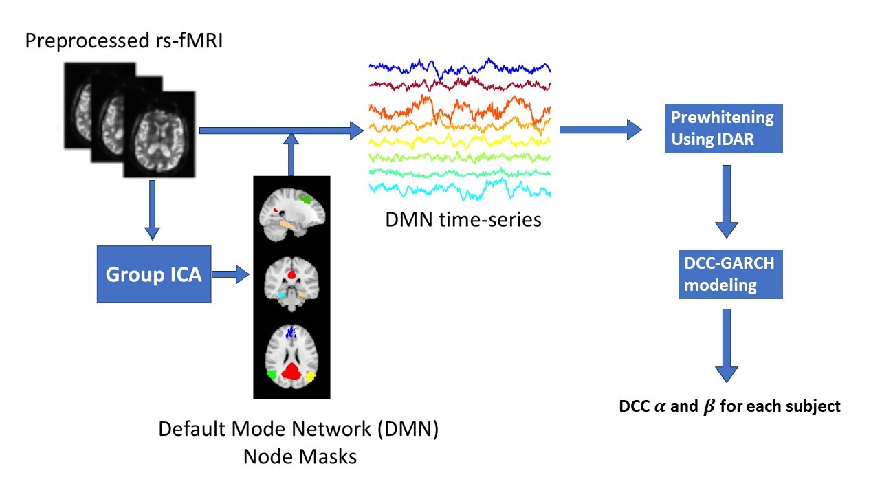
Figure1 illustrates the details of our analysis pipeline. The collected rs-fMRI data undergoes standard preprocessing.⁴¹ Next, we compute time series observations for each node in the DMN. Masks for the DMN nodes were created through group independent component analysis (Group ICA), implemented using FSL MELODIC.⁴² Then, the DCC-GARCH model quantifies the dynamic FC for each subject. Finally, we conduct a group comparison analysis to investigate the differences in dynamic connectivity patterns between AD patients and control subjects.

Figure 1.Flowchart of the analysis procedure.

Study Sample and Data

In this study, we included 87 subjects (mean age = 74 yr, range = 54 to 91 yr). All participants enrolled in University of Washington Alzheimer’s Disease Research Center (UW ADRC, NIH P50 AG005136) Clinical Core, and were recruited with either normal cognition or mild cognitive impairment. All MRI data were acquired with the same protocol for all subjects, using a research-dedicated 3T Philips Achieva scanner equipped with a 32-channel receiver coil. During the scanning session, subjects were instructed to lie in the scanner with their eyes open while wearing a Pearl-Tec™ Crania to minimize head motion.

MRI Data

For registration purposes, we acquired 3D T1 data from all participants. The 3D structural images were obtained using a conventional MPRAGE sequence with the following parameters: spatial resolution = \(1 \times 1 \times 1 {\text{ mm}}^3\), 150 slices, flip angle = 8, TR/TE = 8.8/4.6 ms, SENSE acceleration factor = 2, and matrix size = \(256 \times 256 \times 176\).

Rs-fMRI data was collected using axial whole-brain multi-echo \(T2^\ast\)-weighted sequence over a 10-minute scan period. These images used 3.5 mm isotropic voxels and had TR/TEs of 2,500/9.5, 27.5, and 45.5 ms. Following this, we carried out motion correction using FSL’s MCFLIRT software.⁴² Non-brain matter was then removed using the FSL Brain Extraction Tool.⁴² The multi-echo Blood-Oxygenation-Level-Dependent (BOLD) data were then processed using AFNI’s specialized module TEDANA, for multi-echo planar imaging and analysis with ICA (ME-ICA). TEDANA allows for the differentiation between BOLD (neuronal) and non-BOLD (artifact) components, leveraging the characteristic linear echo-time dependence of BOLD T2 signals.⁴³ This approach produced recombined images optimally weighted across the three echo times, along with ME-ICA-denoised time series and spatial component maps. Subsequently, the data were co-registered to T1 images using FSL. After that, high-pass temporal filtering was applied, and the global signal and motion parameters were regressed from the data.⁴¹

Pre-whitening

To apply the DCC-GARCH model for analysis of BOLD fMRI data, we performed an additional pre-processing step to remove the serial correlation of the BOLD fMRI time series. Although this data pre-processing step has not been sufficiently discussed in the existing literature, the DCC-GARCH model assumes that time series data, after mean signal removal, exhibit no serial correlation (see also Section 2.2.2). Therefore, it is important to ensure the time series have been properly whitened.

To whiten the data, standard software tools commonly fit an Autoregressive Moving Average (ARMA) model^44,45 before fitting a DCC-GARCH model. However, ARMA models often fail to fully address serial correlations, particularly in short-TR fMRI data.⁴⁶ To address this limitation, we use the recently-proposed IDAR approach⁴⁶ as a pre-processing step. The IDAR method effectively mitigates residual serial correlations, ensuring that the data satisfy the DCC-GARCH model’s assumption.⁴⁶ This rigorous preprocessing enhances the validity and reliability of the DCC-GARCH model in capturing dynamic FC.

CSF Measurements

CSF samples were collected via lumbar puncture from all subjects. Levels of \(A\beta42\) and \(A\beta40\) in CSF samples were measured using multiplex bead assays (Luminex xMAP) run on the Luminex 200 instrument according to the manufacturer’s instructions.⁴⁷ Based on their CSF \(A\beta42/40\) ratio, we divided the subjects into two groups: \(A\beta+\) and \(A\beta-\), using the internally determined cut-off threshold of 0.11.⁴⁸ Using this threshold, 25 subjects with CSF \(A\beta42/40<0.11\) are classified as \(A\beta+\) AD patients, and the rest 62 subjects are \(A\beta-\) control subjects.

Group-level Analysis

For each FC network, we calculated two sets of FC measures from the rs-fMRI dataset: static network modeling approach (assuming stationarity) using dual regression, and dynamic network modeling approach using DCC-GARCH. Next, we explain the two modeling approaches.

Static FC: Dual Regression

We estimated individual static FC within the DMN using the ICA dual-regression method.^33,34 To this end, we performed the following analyses:

1. Group-level ICA: We performed ICA on concatenated rs-fMRI data from all subjects to generate a group-level spatial map representing the shared DMN across the cohort.

2. Spatial regression: The group-level DMN map (denoted \(\mathrm{DMN}_G\)) was used in a spatial regression, \[ X_i = \mathrm{DMN}_G \times A_i + e_i,\tag{1}\] where \(X_i\) represents the rs-fMRI data of subject \(i\). In this step, \(\mathrm{DMN}_G\) serves as the spatial regressor, and the resulting vector \(A_i\) contains the relevant individual regression weights in the time domain.

3. Temporal regression: Estimated temporal regression weights (\(A_i\)) were then used as regressors in a second-stage regression, \[ X_i = A_i^\top \times\mathrm{DMN}_i + e_i,\tag{2}\] applied to the subject’s rs-fMRI data. This regression yields \(\mathrm{DMN}_i\), a spatial map containing regression weights that quantify the subject-specific static FC within the DMN.

Following ³⁴, the maps obtained from Eq. 2 were used as an aggregate subject-specific measure of static FC within DMN. Higher static FC measures (in absolute value) imply a stronger average FC throughout the scan duration.

Dynamic FC: DCC-GARCH

We estimated the dynamic FC network of DMN nodes using the DCC-GARCH model. The following eight DMN nodes were used in this study: left and right superior frontal gyrus (SFG), medial prefrontal cortex (MPFC), posterior cingulate cortex (PCC), left and right parahippocampal cortex (PHC), left and right posterior inferior parietal lobule (pIPL). We extracted the corresponding time series for each of the 8 nodes by averaging the measured signals over the node mask voxels obtained from Group ICA. Before performing the dynamic network analysis, we applied IDAR-based pre-whitening procedure to each time series to remove the serial correlations.⁴⁶

We first explain the formulation of the DCC-GARCH model. Suppose we have a multivariate time series \(\{X(t)\}_{t=1}^T\) with \(X(t) \in \mathop{\mathbb{R}}^m\). The time series can be decomposed into a mean component \(\mu(t)\) and a residual component \(\epsilon(t)\): \[\begin{aligned} X(t) = \mu(t) + \epsilon(t), \quad t=1, \dots, T. \end{aligned}\] The mean process \(\mu(t)\) can be modeled as a constant or with a time series model. Here we use a constant mean component. The residual component, \(\epsilon(t)\), is modeled as \(\epsilon(t) = H_t^{1/2}z_t\), where \(z_t\) is a white noise process with variance \(I_m\). The conditional covariance matrix \(H_t\) conditions on the past information up to time \(t-1\). The residual component model indicates \(\epsilon(t)\) is serially uncorrelated, even though it is still serially dependent.

The DCC-GARCH model assumes

\[\begin{aligned} H_t=D_tR_tD_t, \end{aligned}\]

where the dynamic conditional covariance matrix, \(D_t = \mathop{\mathrm{diag}}\left( \{d_{l,t}\}_{l=1}^{m}\right)\), is a diagonal matrix with time-varying standard deviations \(d_{l,t}\) along its diagonal; \(R_t\) is the dynamic conditional correlation matrix that represents the dynamic FC among brain nodes. The dynamic standard deviations, \(d_{l,t}\), are usually modeled by a GARCH(1,1) process: \[\begin{aligned} d_{l,t} = \theta_{l,0} + \theta_{l,1}\left[\epsilon(t)\right]_l^2 + \theta_{l,2} d_{l,t-1}, \quad l=1, \dots, m. \end{aligned}\]

Higher-order GARCH models, denoted GARCH(\(p\), \(q\)), can also be used to model dynamic standard deviations. In this more general case, \(p\) denotes the number of past variances considered, while \(q\) denotes the number of past squared errors considered in the model. The GARCH(1,1) model corresponds to the special case where a single value of past variance and a single past standard error are considered in the model. Although higher order GARCH models can be used for dynamic standard deviations, the GARCH(1,1) model is usually adequate.^39,49 Moreover, while higher-order models may provide more expressivity, fitting such models would require larger number of observations, and higher-order GARCH models may suffer from over-fitting when the number of observations is not large enough. We therefore focus on the GARCH(1,1) model.

The dynamic correlation matrix is modeled by

\[\begin{aligned} R_t = {Q^*_t}^{-1/2} Q_t {Q^*_t}^{-1/2} \end{aligned}\] where \(Q^*_t = \mathop{\mathrm{diag}}(Q_t)\) is the diagonal matrix with the diagonal elements of \(Q_t\), and \[\begin{aligned} h_t & = D_t^{-1}\epsilon(t), \\ Q_t & = (1-\alpha-\beta)\overline{Q} + \alpha h_{t-1}h_{t-1}^\top + \beta Q_{t-1},\\ \overline{Q} & = \frac{1}{T} \sum_{t=1}^{T} h_{t-1}h_{t-1}^\top. \end{aligned}\]

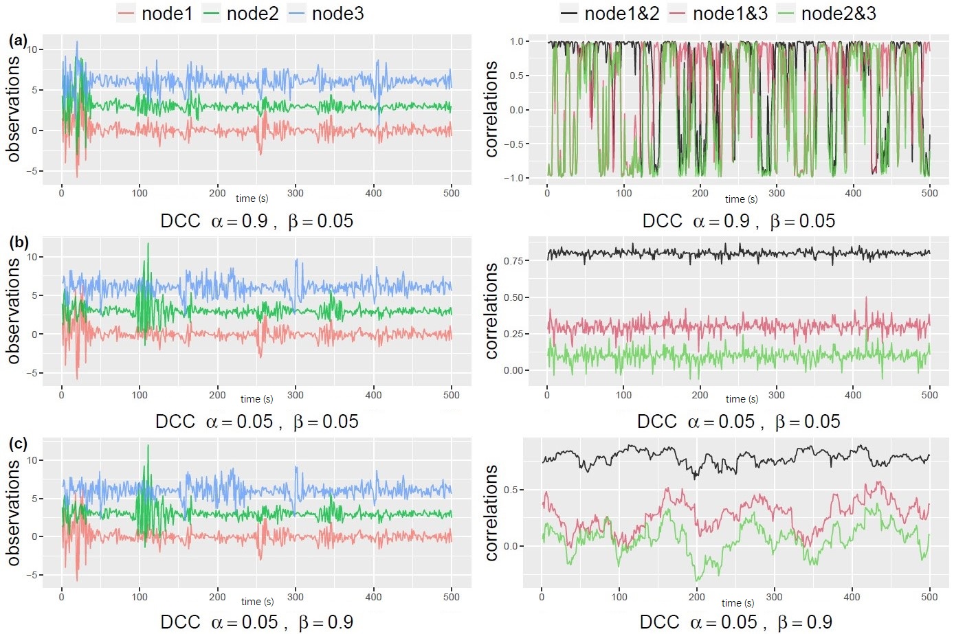
This formulation ensures a proper correlation matrix \(R_t\) that is positive-definite with diagonal entries equal to 1. The two parameters, \(\alpha\) and \(\beta\), characterize the temporal dynamics in the correlation network: \(\alpha\) represents how the correlation matrix dynamically varies as a response to new stimulates, and \(\beta\) quantifies the degree of dependence of the correlations on their past values. To help understand the types of dynamic changes captured by each of the parameters, in Figure 2 we use simulated data to illustrate the dynamic profile of correlations in a 3-node network. To generate the data from a DCC-GARCH model, we employed the R function simulateDCC from the ccgarch2 package (V0.0.0-42, ⁴⁴). For the simulations shown in Figure 2, we set the residual covariance matrix as

\[ \begin{aligned} \left( \begin{array}{ccc} 1 & 0.8 & 0.3 \\ 0.8 & 1 & 0.1 \\ 0.3 & 0.1 & 1 \end{array}\right). \end{aligned} \]

Additionally, for the GARCH(1,1) model of the dynamic standard deviations, we set all the coefficient parameters to \(0.5\). As shown in the plots, both \(\alpha\) and \(\beta\) being small leads to stable correlations that resemble white noise (Figure 2b). Conversely, when \(\alpha\) is small and \(\beta\) is large, the correlation pattern becomes “sticky”, changing slowly over time (Figure 2c). On the other hand, large values of \(\alpha\) and small values of \(\beta\) generate rapid changes in correlations over time (Figure 2a). It is important to highlight that the dynamic profile of the correlations cannot be identified through simple visual examination of the observed signals. This underscores the necessity of employing appropriate models to accurately capture the temporal dynamics.

Figure 2.Illustration of the simulated dynamic profile of correlations with respect to different \(\alpha\) and \(\beta\) values. We simulate three sets of time series observations for a 3-node network based on DCC-GARCH model. Each set has different parameter values for (\(\alpha,\beta\)). The left side plots show the simulated signals from three nodes, and the right side plots show the dynamic profile of the corresponding pairwise correlations from the DCC-GARCH model.

To analyze the dynamic correlation profiles from the fMRI data, the DCC-GARCH model was estimated via maximizing the quasi-likelihood, using the procedure implemented in the R package rmgarch.⁵⁰ After obtaining the subject-level estimates for the dynamic characterization parameters \(\alpha\) and \(\beta\), we collected the estimates and conduct a two-sample t-test for a group-level comparison between \(A\beta+\) AD patients and \(A\beta-\) control subjects. We tested for group differences at 0.05 significance level.

Results

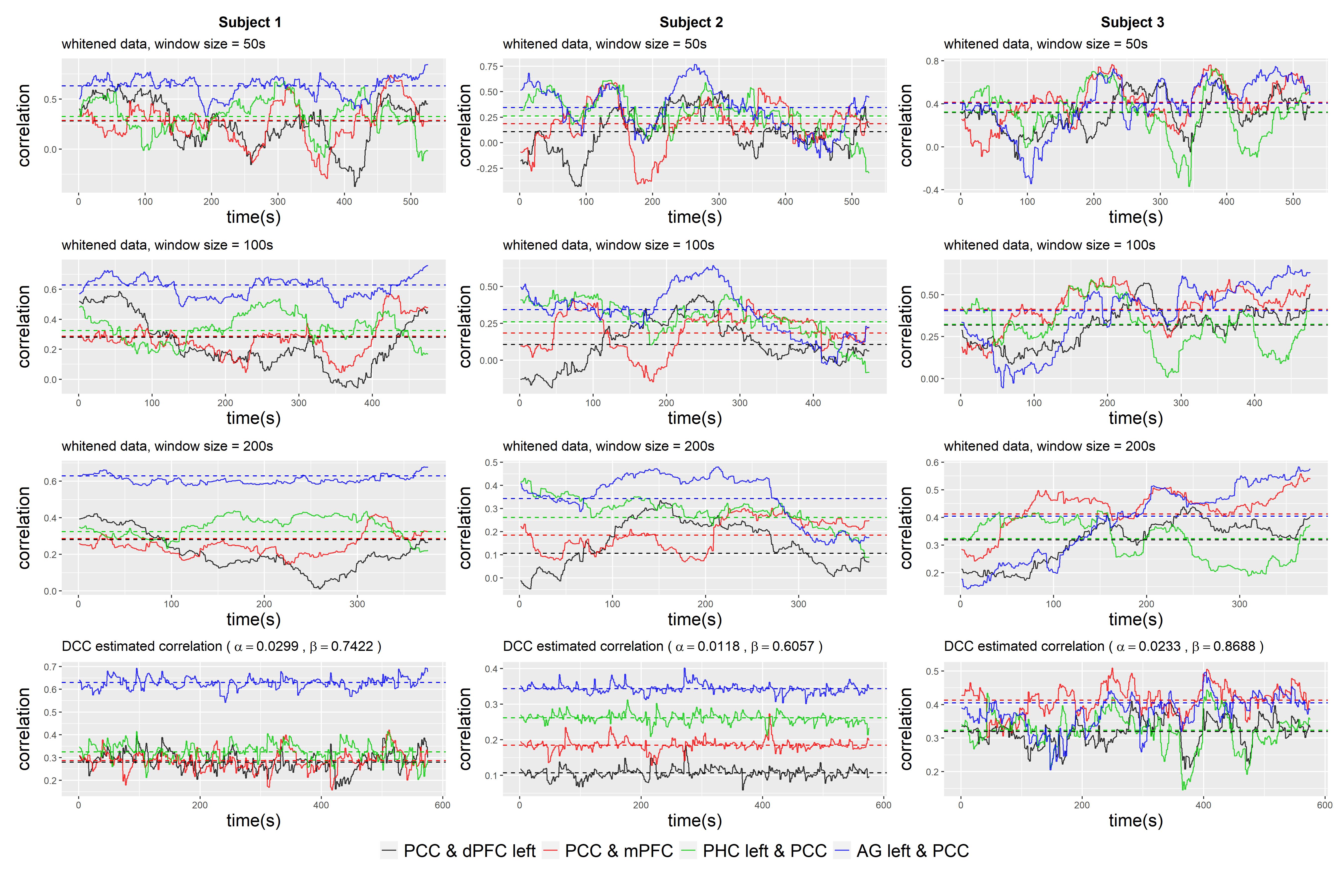
We begin by visualizing the dynamic correlation profile of an example subject based on the raw and whitened fMRI data using the sliding window approach. In this approach, we employed a simple rectangular window function. For the purpose of exposition, we focused on visualizing the correlations between specific pairs of brain nodes, namely PCC and SFG left, PCC and MPFC, PCC and PHC left, and PCC and pIPL left. As suggested in,⁵¹ the choice of a suitable minimum window length is influenced by the minimum frequency of the fMRI measurement. In our dataset, a window length of 100 seconds (equivalent to 50 data points) seemed appropriate. For comparison, we also included window lengths of 50s, 200s, and 400s. As depicted in Figure 3, the observed correlations exhibited temporal variability. The variability could become substantial, resulting in correlations that not only change sign, but also exhibited a large amplitude that can be more than twice the magnitude of the static correlation measurement. However, the magnitude of this variation was highly dependent on the window length, making it challenging to distinguish between genuine underlying dynamics and spurious fluctuations. Comparing the correlation profiles estimated from raw and whitened data, we observed that the dynamic pattern was not significantly altered by the whitening procedure. However, there was a notable decrease in the correlation between PCC and MPFC for this subject, with the static correlation measurement decreasing from 0.51 to 0.33.

Figure 3.The dynamic correlation profile of three example subjects, using the whitened data, based on the sliding window approaches (top three rows) and the DCC-GARCH approach (last row). The sliding window approach applies the rectangular window function at window length = 50s, 100s, 200s. We visualize the correlation profile of four chosen brain node pairs. The dashed lines represent the standard static correlation coefficient for each node pair, computed using data from the full time course.

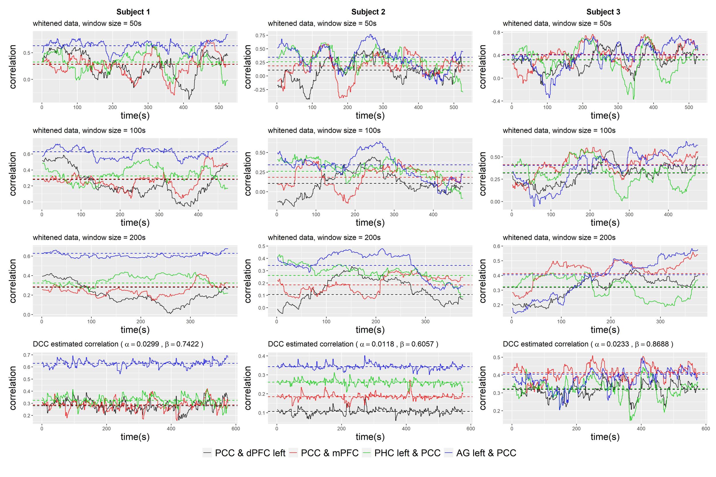
Figure 3 compares the sliding-window-based correlations with the correlation profiles based on the estimated DCC-GARCH model. Three example subjects whose correlation profiles vary are shown. The correlations calculated with the DCC-GARCH model show more noticeable differences among the subjects. Notably, the estimated correlation trajectories capture certain variation patterns identified by the sliding window approach. For instance, in subject 1, large drops in the correlations between PCC and SFG left were observed towards the end of the observation period.

By fitting separate DCC-GARCH models to each subject in the dataset, we observed significant group differences at 0.05 level in terms of the subject-level dynamic characterization parameter \(\alpha\) between \(A\beta-\) control subjects and \(A\beta+\) AD patients (Figure 4). The group difference in dynamic characterization parameter \(\beta\) was marginally significant at the 0.1 level. In general, \(A\beta+\) AD patients had lower \(\alpha\) values and higher \(\beta\) values, indicating less responsiveness to outside stimuli and more dependence on the previous brain’s connectivity status in the DMN compared to the healthy subjects. In contrast, the static FC measurement based on standard dual-regression ICA analysis (Figure 4) did not show significant group difference.

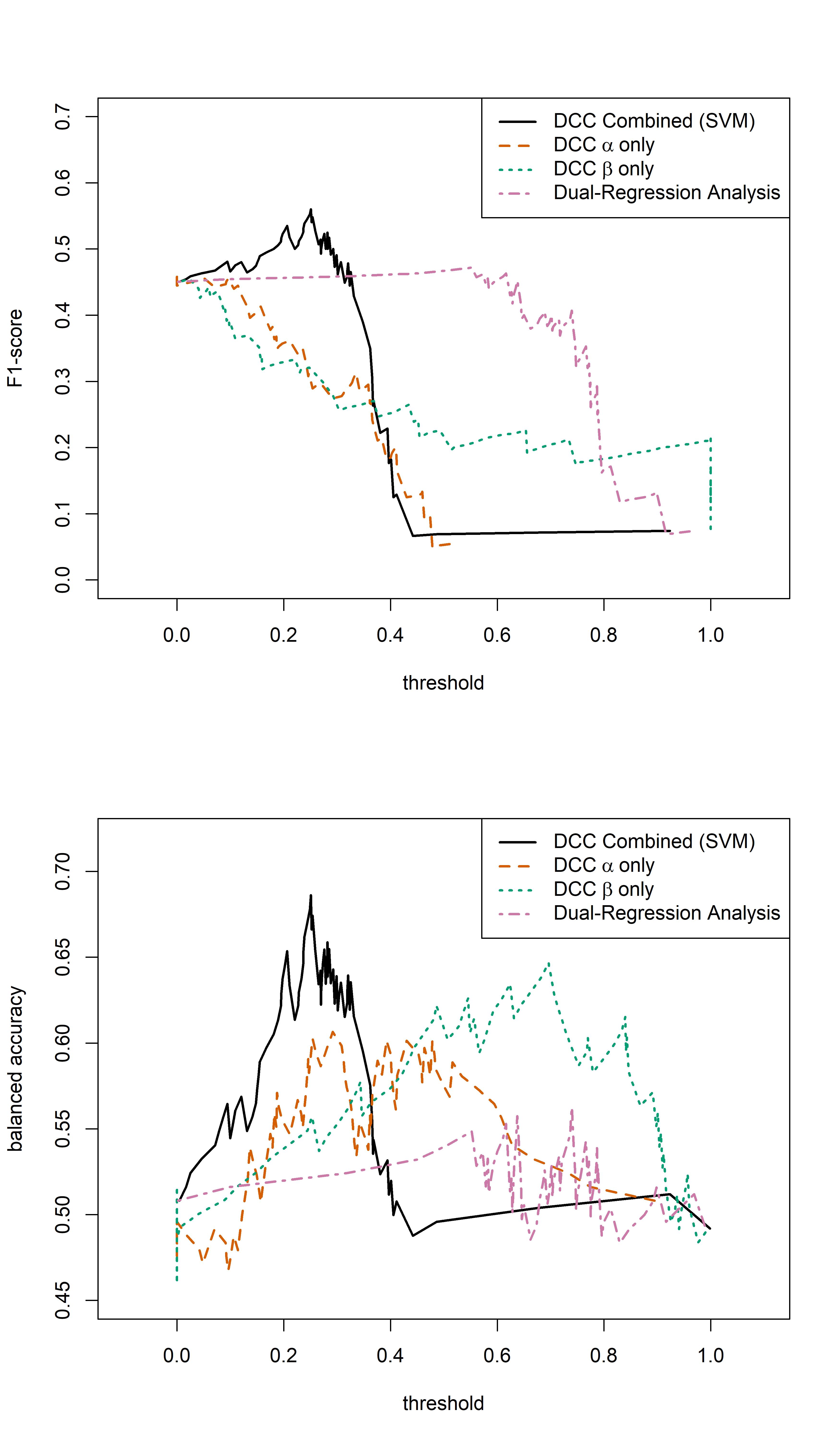
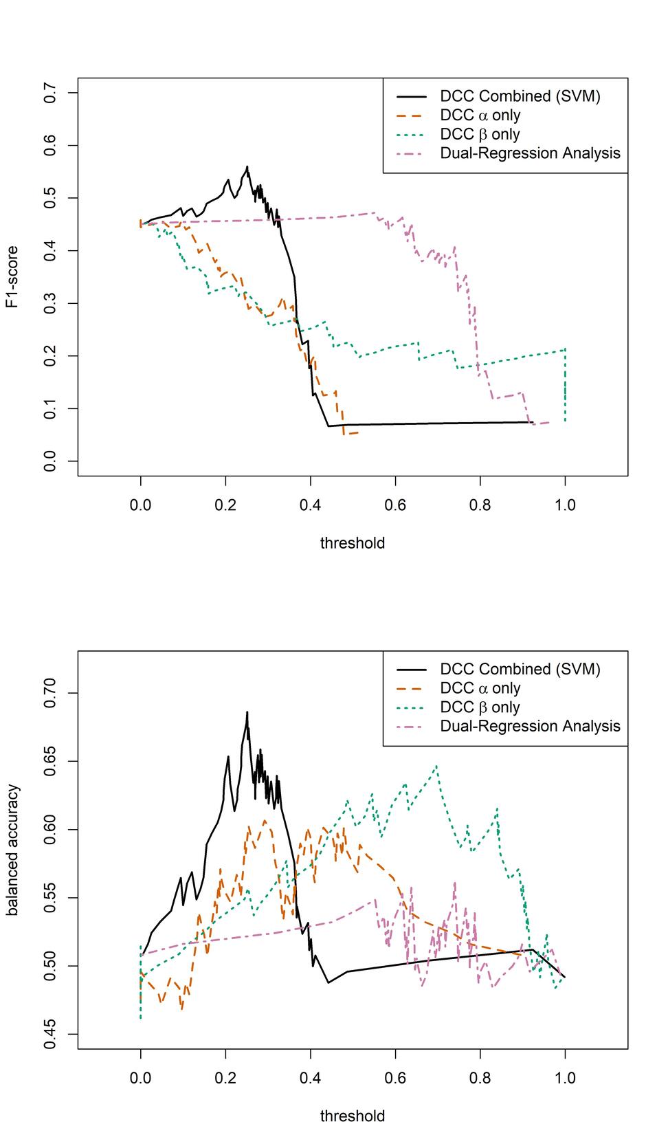
We then evaluated the sensitivity and specificity of the estimated DCC-GARCH parameters in identifying AD patients (Figure 5). To obtain a comprehensive picture of models’ performances, we also examined the F1-score, which is the harmonic mean of the precision and recall, and balanced accuracy, which is the average of sensitivity and specificity (Figure 6). Classification of subjects as \(A\beta+\) was performed using varying threshold values applied to the estimated DCC-GARCH parameters \(\alpha\) and/or \(\beta\). By sweeping thresholds from 0 to 1, we generated ROC curves and calculated their AUC values (Figure 5), and corresponding F1-score and balanced accuracy in Figure 6. For clarity, both the predictions and thresholds are scaled to range from 0 to 1, where higher values indicate \(A\beta+\) cases. In the “combined” approach, where both \(\alpha\) and \(\beta\) values were used for classification, we implemented a Support Vector Machine (SVM) with a radial kernel. The tuning parameters (\(\gamma\) and regularization constant \(C\)) were optimized to maximize the AUC through 10-fold cross-validation. When used independently for classification, the \(\alpha\) and \(\beta\) parameters demonstrated moderate power to identify AD patients, each with an AUC of approximately 0.6 and balanced accuracy peaking between 0.6 and 0.65. However, their F1-scores remained relatively low. In contrast, combining both \(\alpha\) and \(\beta\) parameters improved diagnostic performance, resulting an AUC of 0.7 and maximum F1-score of 0.56—the highest among all methods across a wide range of threshold values. On the other hand, the static FC measurement of average DMN strength computed from dual-regression ICA analysis exhibited poor classification performance in terms of ROC curve, AUC, and balanced accuracy. Although its F1-score was stable and moderate among all methods, its peak value did not match the performance achieved by combining both DCC parameter values.

Figure 4.(a) Boxplots of estimated DCC-GARCH \(\alpha\) and \(\beta\) parameters calculated using the proposed method for all subjects. Each dot represents the parameter estimate for a single subject. Subjects were divided into two groups based on their CSF \(A \beta\) profile: 1) AD patients (CSF \(A \beta 42 / A \beta 40<0.11\) ), and 2) control (CSF \(A \beta 42 / A \beta 40 \geq 0.11\) ). p-values of two-sample t-test for group differences in parameter estimates are reported. (b) Boxplots of average static FC in DMN, calculated using dual-regression ICA analysis.

Figure 5.ROC curves and AUC for identifying \(A \beta+\) AD patients based on estimated DCC-GARCH parameters. The ‘DCC \(\alpha\) only’ and ‘DCC \(\beta\) only’ curves are based on thresholding the estimated \(\alpha\) or \(\beta\) values separately, the ‘DCC Combined’ ROC curve is yielded from using \(\alpha\) and \(\beta\) values via the SVM approach. The ‘Dual-Regression Analysis’ ROC curve is based on average DMN strength computed from dual-regression ICA analysis.

Figure 6.F1-score and balanced accuracy curves for identifying \(A \beta+\) AD patients based on estimated DCC-GARCH parameters. The ‘DCC \(\alpha\) only’ and ‘DCC \(\beta\) only’ curves are computed based on thresholding the estimated \(\alpha\) or \(\beta\) values separately, the ‘DCC Combined’ ROC curve is yielded from using \(\alpha\) and \(\beta\) values via the SVM approach and thresholding the corresponding outputs. The ‘Dual-Regression Analysis’ curve is based on thresholding average DMN strength computed from dual-regression ICA analysis.

Discussion

Our study sheds light on the importance of considering dynamic network configurations and the limitations of static measures of FC when searching for biomarkers for AD. To capture the temporal dynamics of brain network connectivity, we proposed using a DCC-GARCH model. Proper pre-processing steps, especially an effective pre-whitening procedure to eliminate serial correlations, are necessary for the validity of applying the DCC-GARCH model, which ensures the model assumptions are met. By addressing these key issues, our findings contribute to the understanding of FC analysis in AD research and offer insights into the development of non-invasive and widely available biomarkers for the early detection of the disease. The results of our study indicate that the proposed DCC-GARCH modeling approach for dynamic FC in the DMN is sensitive to the CSF \(A\beta\) status. Specifically, the dynamic FC measurements of \(A\beta+\) AD patients seem to exhibit higher lagging dependency and reduced responsiveness to new information compared to healthy controls. The resulting DCC-GARCH model parameters show reasonable power in identifying \(A\beta+\) AD patients in the population, indicating its potential as a sensitive biomarker for early detection of AD based on \(A\beta\) deposition. We anticipate that with a larger number of subjects, the differences between the two groups would become more significant. Additionally, we expect that increased sample size would lead to better predictability of our model.

The results in Section 3 indicate that, depending on the evaluation criterion, the predictive performance of the dynamic and static FC models depends on the threshold used for classification: When comparing the AUC values obtained over all thresholds, the proposed prediction model based on both DCC-GARCH parameters offers clear advantages over the model based on static FC measures (obtained via dual regression). However, in terms of the \(F_1\) measures, the proposed method offers an advantage over a limited range of thresholds, whereas the comparison of balanced accuracies paints an intermediate picture: the proposed method offers improvement over a wider range of thresholds. Aside from the predictive performance, the DCC-GARCH model provides a plausible description of the temporal dynamics in the DMN, considering the data from the perspective of autoregressive dependency. While it may not represent the true or best model for describing the brain mechanism, it effectively captures important variation patterns identified by the sliding-window-based approach. The estimated dynamic functional correlation profiles using the DCC-GARCH model tend to be more stable and more concentrated around the static correlation measurement compared to the sliding-window-based approach, reflected in smaller standard deviations over the time course. Further investigation should explore alternative perspectives, such as network topology or identifying change points in correlation profiles, to gain deeper insights into potential group differences. By examining multiple aspects, we can enhance our understanding of the dynamic FC alterations associated with AD pathology and uncover more sensitive biomarkers for early detection.

In summary, our study provides valuable insights into the analysis of dynamic FC in AD and the potential for developing biomarkers for the disease. The utilization of the DCC-GARCH model offers a promising approach to capturing the temporal dynamics of brain network connectivity. Future research should focus on validating our findings in larger cohorts of independent subjects and exploring additional factors that may differentiate the dynamic correlation profiles observed between \(A\beta+\) patients and \(A\beta-\) individuals. Further research is also needed to investigate how dynamic FC may differentiate individuals across the AD spectrum, both with respect to AD pathology and cognitive function. By continuing to advance our understanding of FC dynamics, we can pave the way for improved diagnosis and monitoring of AD, ultimately leading to more effective interventions and treatments.

Data Availability

Researchers can obtain de-identified raw imaging data by accessing the National Alzheimer’s Coordinating Center (NACC) website, which includes DICOM format raw imaging files and variables from the NACC Uniform Dataset Version 3.0. Additionally, investigators with an IRB-approved study and a designated UW ADRC collaborator may be granted access to the UW ADRC Imaging and Biomarker Core database. The imaging data utilized in this study is available in BIDS format and is stored on an XNAT platform in the UW Integrated Brain Imaging Center. For inquiries, please reach out to Dr. Thomas Grabowski MD, Lead of the Imaging and Biomarker Core at UW ADRC.

Funding Sources

This work was supported by the ADRC grant P30 AG066509. Ali Shojaie was partially supported by grant R01-GM133848. Hesamoddin Jahanian was partially supported by NIH grant K01 AG071798.

Conflict of Interest

The authors declare no competing interests.