Fast and scalable joint-LORAKS reconstruction and data-driven sampling optimisation of high-dimensional MRI datasets using a GPU-accelerated and learning-free differentiable framework: PyLORAKS

Introduction

Magnetic resonance imaging (MRI) is an indispensable tool in medical diagnostics, offering detailed images of the human brain’s internal structures. However, the acquisition of high-quality MR images is often constrained by the trade-off between scan time and image resolution. High-resolution imaging in particular requires large k-space acquisition matrices, which in turn depend on the collection of vast data.

Parallel Imaging (PI) techniques like generalised autocalibrating partially parallel acquisitions (GRAPPA)¹ and sensitivity encoding (SENSE)² are routinely used in multichannel receive coil setups to decrease scan time by undersampling k-space acquisition. Promising reconstruction techniques have been demonstrated relying on low-rank matrix completion, like low-rank matrix modelling of local k-space neighbourhoods (LORAKS).³ LORAKS exploits the low-rank properties of specific operator matrices built from small neighbourhoods around each k-space point to facilitate reconstruction. The neighbourhoods can be extended by combining available channels to reconstruct multichannel data.⁴

Many MRI acquisitions depend on sequence variations to produce different contrasts, such as multi-echo temporal signal weighting^5–8 or diffusion gradient weighting.^9,10 Algorithms to handle reconstruction jointly across contrasts have already been demonstrated.^11,12 In particular, joint-echo reconstruction using a Joint-LORAKS (J-LORAKS) framework has been shown to outperform GRAPPA-based variants in image reconstruction quality.¹³

Despite its effectiveness and improvements to the original algorithm,¹⁴ such as AC-LORAKS using an autocalibration (AC) region to speed up computations,¹⁵ the computational demands of J-LORAKS pose significant challenges. Commonly, a singular value decomposition (SVD) operation is used to enforce low-rank structure. SVD scales quadratically in time and linearly in memory computation complexity.^16,17

The structured matrices used in LORAKS scale linearly with the number of receive channels and contrasts (in modern scan settings: \(\geq 32\) receive channels, \(\geq 2\) contrasts), hindering reconstruction optimisation by high computational time and restricting high-resolution reconstruction by infeasible memory requirements. For example, we carried out the joint-reconstruction of an MRI scan with an acquisition matrix of \(280 \times 280\) in plane, 100 slices, 32 receive channels, and three echoes on a modern compute server with the recent LORAKS software implementation.¹⁸ The time consumed is > 3 d to process the whole dataset, while the requirement on the available system memory (RAM) is around 170 GB. Similarly, in comparison to other reconstruction techniques, LORAKS required the longer reconstruction times, without even including its computationally extensive phase constraint formalism or joint-reconstruction capabilities.¹⁹

Another challenge of LORAKS is the choice of the algorithm parameters (regularisation weighting \(\lambda\) and rank \(r\)), which are not known a priori and require careful balancing. Influence of the rank parameter \(r\) is commonly gained empirically by visual data assessment after reconstruction.^14,20,21 Especially for J-LORAKS, inherent high computational cost and slow computation speed hinder brute force methods or manual user selection. Automation of the parameter choices has been proposed using Stein’s unbiased risk estimator (SURE),²² in conjunction with coil sensitivity map estimation for a SENSE-based PI reconstruction.²³ Similarly, the LORAKS rank parameter has been subjected to SURE optimisation using compressed-sensing, total variation, and wavelet regularisation,²⁴ which further increases the computational needs upon reconstruction, with the time feasibility depending on the J-LORAKS reconstruction performance.

Multiple reconstruction frameworks and LORAKS extensions have been suggested to address its poor scaling and computational performance, utilising specific optimisation formulations or additional constraints.

A fast convolutional procedure (HICU) tailored to low-rank matrix completion introduced computational optimisations regarding gradient computation and precise step size estimation in its iterative solving.²⁵ Furthermore, randomised SVD (rSVD) was used to approximate low-rank deficiency,²⁵ offering improved stability and parallel computing.²⁶

Despite speedup and memory reduction, HICU only extends the LORAKS compact support constraint, not using the additional phase-constraint, which was found to be superior in a number of applications.²⁷ Nevertheless, substituting the core matrix-decomposition with rSVD proves beneficial,^17,28 and recent variants like subspace-orbit rSVD¹⁶ or randomised nullspace approximation (RAND-NS)²⁹ may yield further efficiency gains for large matrices encountered in J-LORAKS.

Efficient parallelised computations, specifically accessing GPUs, were used in a plethora of variations either replacing or mimicking the regularisation term through deep-learning algorithms.^30–32 In this context the iterative and convolutional nature of LORAKS operators, AC-LORAKS in particular, allows viewing LORAKS itself as an autoregressive network. Thus, AC-LORAKS was implemented as a network building block in an autoregressive ensemble approach for k-space interpolation.³³ Although implemented in PyTorch,³⁴ graphics processing unit (GPU)-specific details were not provided, computation times were not reported, and the achieved fidelity comes at the expense of computational overhead by adding multiple other ensemble blocks.

LORAKI replaced the explicit computationally demanding low-rank enforcement by a parametric recurring neural network (RNN).³⁵ The LORAKS prior thus is encoded in the RNN weights rather than using an explicit mathematical formulation. Furthermore, the RNN needs to be trained, which was reported with runtimes of 1 h for rather small slice dimensions (\(256 \times 187\)) and \(12\) channels.³⁵ Usually, for inference, the computation time of the trained model is much faster and the process might be subject to similar optimisations shown for the original RAKI implementation,³⁶ but to the authors’ knowledge, no such implementation was made available at the time of this study.

Our implementation uses PyTorch for parallel execution on GPUs, previously used to accelerate MRI reconstruction.^37–39 PyTorch’s automatic differentiation engine⁴⁰ enables efficient gradient computation through the entire reconstruction pipeline. It allows treating the LORAKS reconstruction itself as a differentiable computational graph. Such a traceable LORAKS constraint can be combined with other regularisation terms,⁴¹ or as a building block for physics-informed deep learning^42,43 or generative AI models⁴⁴ and allows novel optimisation approaches.

However, in our implementation, we intended to keep the inherent mathematical rigour of the low-rank mechanism building a learning-free framework, as the black-box character of deep-learning methods poses challenges in interpretability and evaluation of the models.⁴⁵

In this paper, we present an enhanced LORAKS implementation designed to overcome computational limitations, enabling efficient joint-reconstruction of undersampled, multichannel, multi-contrast MRI images. We develop PyLORAKS, a Python-based LORAKS algorithm using PyTorch, enabling GPU utilisation. Further, we changed the operator construction in order to enable efficient linear memory access, and ensured PyLORAKS reconstruction similarity to, and benchmarked against the latest publicly available LORAKS MATLAB⁴⁶ version.¹⁸

To extend the LORAKS mechanism, we incorporated and tested recent rSVD methods and introduced an automatic backpropagation feature. Additionally, we introduce batching strategies for efficient leveraging of multichannel, multi-contrast data redundancy to enable joint-reconstruction of high-resolution data with feasible time and computational constraints.

Furthermore, we demonstrate a number of exemplary implications of our framework for MRI research. For a specific 2D multi-echo acquisition, we evaluate the choices of LORAKS parameters \(\lambda\) and \(r\) on joint-reconstruction to optimise the reconstruction and provide general recommendations for the parameter settings in PyLORAKS. Additionally, we demonstrate the ability for acquisition optimisation using our framework by computing an optimised sampling scheme and showing increased reconstruction quality, which is transferable to reduced scan time in high-resolution MRI acquisitions.

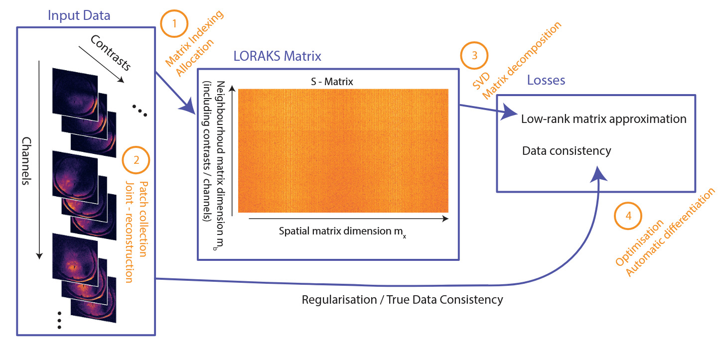
The steps involved in LORAKS reconstruction, together with modifications and additional features presented in this study, are sketched in Figure 1 for reference.

Figure 1.LORAKS reconstruction implementation steps.

The input data (left column) is processed per 2D-slice and arranged to combine multiple contrasts (2). Dependent on the projected memory size of the algorithm, the combined contrast and channel dimension is batched using a channel-correlation-based clustering (described in the data combination and batching subsection). The Casoratti-style LORAKS matrix can be built by indexing of the combined input data (1). The indexing was designed to allow linear memory usage and avoid loops for computational efficiency. The LORAKS matrix is used to enforce a low-rank constraint which is using a rank-revealing decompoisition like SVD. With increasing LORAKS matrix sizes, due to high-resolution input data or joint reconstruction of many channels and/or contrasts, this method is computationally costly. Huge matrix sizes can effectively be subjected to low-rank matrix completion using randomised methods (3). Finally, the used framework allowed the implementation of AI-style backpropagation which can be used for data-driven sampling optimisation (4).

Materials & Methods

LORAKS can be regarded as a two-fold process: (1) building the LORAKS neighbourhood matrix (from k-space data \(\boldsymbol{k}\)) and (2) optimising a loss function to drive a low-rank matrix constraint and ensure data fidelity. The reconstruction of the 5D k-space data \(\boldsymbol{k} \in \mathbb{C}^{N_x \times N_y \times N_z \times N_c \times N_e}\), consisting of three spatial dimensions (\(N_{x,y,z}\)), multichannel and multi-contrast data (\(N_{c,e}\)), with missing and zero-filled entries, becomes the following minimisation problem³:

\[ \boldsymbol{\hat{k}} = \min_{\boldsymbol{k} \in \mathbb{C}^{R}} ||{\boldsymbol{F}\boldsymbol{k} - \boldsymbol{d}}||_{2}^2 + \lambda J_r(\boldsymbol{P}(\boldsymbol{k}))\tag{1}\]

Here, \(\boldsymbol{F}\) is the sampling operator, which neglects missing entries and \(\boldsymbol{d}\) is the actual acquired k-space samples. \(J_r(\cdot)\) is a nonconvex regularisation penalty that enforces rank \(r\) on its argument. \(\boldsymbol{P}(\cdot)\) is the LORAKS matrix operator, which constructs the LORAKS matrix from the k-space input by collecting neighbourhood patches around each spatial position in \(\boldsymbol{k}\). LORAKS employs distinct types of neighbourhood matrix operators which impose different restrictions on k-space. For example, the C-operator requires limited support, and the S-operator imposes a smooth phase. We restrict the study to LORAKS reconstruction using the S-operator, since empirical findings suggest superior results across a range of applications.²⁷ However, all methods can be applied to the C-operator as well.³ Without loss of generality, assuming \(\boldsymbol{k}\) to be 2D slices of k-space data, we denote the matrix dimensions \(\boldsymbol{S} = \boldsymbol{P}(\boldsymbol{k}) \in \mathbb{R}^{2 m_x \times 2 m_{ce}}\), where the factor of two arises from the S-operator’s conjugate-symmetry construction.

The spatial dimension \(m_x \sim N_x \times N_y\) includes all patches fully contained within the slice, where \(N_{x,y}\) are the slice dimensions. The neighbourhood dimension \(m_{ce}\) depends on the square neighbourhood patch of size \(p_s\). For the multichannel formulation, the channels are concatenated along this dimension, as are the contrasts for a joint-reconstruction setup.¹³ Thus \(m_{ce} = p_s^2 \times N_c \times N_e\), where \(N_{c,e}\) are the numbers of channels and contrasts, respectively. In a typical clinical setting \(N_c\) is around \(16\) or \(32\) and \(N_e\) can be as high as \(10\) depending on the acquisition method. Thus, with a multi-echo acquisition of \(5\) echoes and 32 receive channels \(m_{ce} = 4000\). We set \(m_b = 2 m_{ce}\) for convenience throughout this manuscript. The matrix can be seen in Figure 1, outlining the steps of the approach.

Several methods have been proposed in conjunction with least-square solvers³ to find solutions to the minimisation problem in equation 1. Further computational improvements were made using the approximation¹⁵

\[ J_r(\boldsymbol{P}(\boldsymbol{k})) \sim\|\boldsymbol{P}(\boldsymbol{k}) \boldsymbol{V}\|_F^2, \tag{2}\]

that uses the Frobenius norm for an appropriate choice of the matrix \(\boldsymbol{V}\). When the subsampled k-space contains autocalibration (AC) data, \(\boldsymbol{V}\) can be extracted from the nullspace of the LORAKS matrix built from the AC region \(\boldsymbol{P}(\boldsymbol{k}_\mathrm{ac})\).¹⁵ The properties of the LORAKS matrix and the convolutional structure ingrained in the matrix norm in equation 2 allow for further computational gains by fast fourier transforms (FFT) to find the solution.¹⁴

We restrict this study to the fast AC-LORAKS reconstruction method, focusing on its practical applicability rather than providing an exhaustive comparison. The assumption of available AC data is well justified, since it underlies the majority of parallel imaging strategies, including widely used approaches such as SENSE² and GRAPPA,¹ for which a number of autocalibration methods like FLEET^47,48 exist. However, original loss-solving methods, LORAKS matrix operators (C and S - matrix) and calibrationless P-LORAKS have been included in PyLORAKS. Our motivation for PyLORAKS was its use for sampling optimisation and sequence development in our research, requiring low computation time to enable fast development cycles. Similar results can be achieved using PyLORAKS with other algorithmic variations as the improvements presented are not specific to the particular algorithmic choice.

Data & Hardware

For evaluation of the algorithm and its features, we used different virtual data and in vivo MRI high-resolution data scans.

Virtual data

Random matrices

To simulate different S-matrix sizes in our experiments testing randomised matrix decomposition methods, we used torch.randn() to create random matrices \(\boldsymbol{\tilde{M}} \in \mathbb{R}^{{m_x} \times m_b}\). We set \(m_x = 86016 = 2 \times 224 \times 192\) as representative spatial LORAKS S-matrix axis for an image slice. The LORAKS neighbourhood dimension (representing concatenated channels and/or contrast) was varied from \(m_b \in \left\{2 \times 200, \ldots, 2 \times 15000\right\}\), using 20 equally spaced values.

Shepp-Logan

For memory and speed benchmarks of the PyLORAKS framework, we used a Shepp-Logan virtual data phantom⁴⁹ to simulate one slice of imaging data.

To vary the neighbourhood dimension \(m_b\) of the LORAKS matrix, we simulated different receive channel coil-sensitivities by placing \(N_c\) 2D Gaussian windows at random points within the imaging slice with a standard deviation of \(\sigma \in \left[\sqrt{N_{x,y}/8 }, \sqrt{N_{x,y}/3}\right]\), where \(N_{x,y}\) is the respective image dimension. The number of receive channels was set to be \(N_c \in \{4, 8, 12, \ldots, 36\}\).

Additionally, we assigned randomised decay rates to the different intensity classes in the Shepp-Logan phantom to generate a Shepp-Logan decay rate map \(R\), which was used to simulate additional \(N_e\) relaxation contrasts. Thus, decay images were created multiplying the phantom by the factor \(e^{(-N_e R(x, y))}\), varying \(N_e \in \{2, 3, 4, 5, 6\}\).

Random Gaussian noise was added to the k-space data of each contrast and channel, respectively, using the torch.randn() function setting torch.manual_seed(0).

The neighbourhood patch size was chosen to be \(p_s = 5\) in PyLORAKS and a radius of \(R=3\) in Matlab for an equal number of patch elements. For the neighbourhood dimension defined by \(m_b = 2 m_{ce} = 2 p_s^2 N_e N_c\), we get \(m_{ce} \in \{400, \ldots, 10800\}\) with varying \(N_c\) and \(N_e\). The spatial dimension of the LORAKS matrix was varied with from \(N_{x,y} = 100\) to \(N_{x,y} = 280\), increasing by \(10\) at each step, and, therefore, \(m_x \in \{10000, \ldots, 78400\}\).

MRI data

For data-driven optimisations regarding the joint-reconstruction data combination and parameter and sampling optimisations, we used high-resolution in vivo data.

Acquisition

All data were acquired on a Magnetom Terra 7 T MRI scanner (Siemens Healthineers, Erlangen, Germany). We used an 8Tx/32Rx channel phased array RF head coil (Nova Medical, Wilmington, MA, USA). Note that the number of transmit (Tx) channels is irrelevant for the reconstruction considerations in this study. The transmit mode was set to Siemens “True Form” to produce a circularly polarized (CP) \(B_1^+\) transmit field. For in vivo data, three participants (two females ages 20 y and 24 y, one male age 37 y) were scanned. The study was approved by the Ethics Commission at the Faculty of Medicine of Leipzig University and written informed consent was obtained.

We acquired a 2D multi-echo spin-echo (MESE) sequence designed using PyPulseq.^50,51 PyPulseq delivered a well-defined raw data stream, and the particular sequence was chosen for convenience to demonstrate multi-echo reconstruction. Additionally, PyPulseq enabled fast manipulation of sampling-scheme routines within the sequence.

We used an echo-train length of 8, an echo-spacing of 7.73 ms and a \(T_R\) of 4.5 s. Fully sampled data was acquired in 17m 15s with an FOV of \(212\text{mm} \times 165 \text{mm} \times 28\text{mm}\) and a matrix size of \(304 \times 237 \times 28\).

Sampling

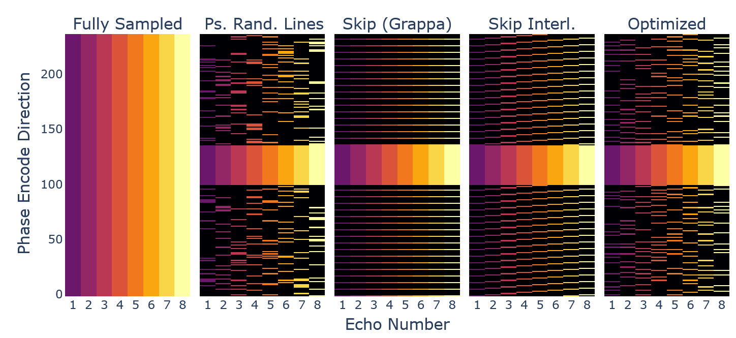
Retrospective undersampling was achieved using different masking of k-space data and zero-filling. The fully sampled dataset served as a reference. We used the following sampling patterns, which can be appreciated in Figure 12:

1. Pseudo-randomised sampling of points from a uniform distribution outside a central spherical AC region, without replacement.

2. Pseudo-randomised sampling of lines along one dimension from a uniform distribution outside the AC region, without replacement.

3. GRAPPA¹ sampling, i.e. skipping of lines outside the AC region.

4. Interleaved skipping of lines outside the AC region with respect to the echo dimension, a GRAPPA-style pattern with a more homogenous coverage across echoes.⁵²

Only the GRAPPA method does not provide complementary sampling across echoes. The other methods capture different k-space lines across the various echoes in coherent or randomised fashion, as it was found beneficial in joint-reconstruction settings.^13,52

For each pattern we created an AC region with 36 central lines. We used an acceleration factor of \(a = 3\) in the data combination experiments. In our parameter optimisation experiments, acceleration factors \(a \in \{2, 3, \ldots 6\}\) were evaluated. For the sampling optimisation experiments we used a factor of \(a = 5\), such that, due to the data size, each echo was sampled using 76 lines.

Evaluation metrics

In all comparison or optimisation experiments involving the in vivo data, we calculated evaluation metrics with respect to the fully sampled data reference. We used normalised mean squared error (NMSE) \(\eta_\text{nmse}\),⁵³ peak signal-to-noise ratio (PSNR) \(\eta_\text{psnr}\),⁵⁴ and the structural similarity coefficient (SSIM) \(\eta_\text{ssim}\).⁵⁴

Compute System

We used a dedicated Linux compute server with a 72-core Xeon Platinum 2.4 GHz CPU (4800 bMIPS) with 1 TB RAM and an NVIDIA l40S GPU with 46 GB RAM in all computational experiments.

Note, computation speed is dependent on used floating point precision (we used 32-bit precision) and the compute system, as well as underlying library implementations and backends. Thus, the presented results might not be directly transferable to other systems or software versions.

Algorithm innovations & technical implementation

We used PyTorch³⁴ (version 2.4.1) and Python (version 3.10) to implement the PyLORAKS MRI reconstruction framework.⁵⁵

We will refer to the original algorithm^3,14 implemented in Matlab⁴⁶ as M-LORAKS. Compared to M-LORAKS, a number of improvements were implemented, which will be outlined in the following sections. Additionally, the reconstruction result was tested against M-LORAKS to ensure comparable results.

Efficient computation and GPUs

In modern computing multiple factors lead to an immense increase in efficiency for vectorised or parallel computations.^56–58 Hence, whenever possible, iterative or sequential loops should be avoided in favour of batched or vectorised operations, which are available in most modern scientific computing libraries. Additionally, using PyTorch, data and most computations can be transferred to GPUs (graphical processor units) for efficient and fast parallel computations. We used CUDA⁵⁹ (version 12.4) and associated libraries (libcublas, libcufft, libcusolver, libcusparse) including vectorised functions for all presented matrix decomposition methods and other linear algebra operations.

Linear indexing for LORAKS matrix operators

M-LORAKS collects the LORAKS neighbourhoods of each k-space position within a circular neighbourhood by sequential iteration through all spatial k-space dimensions. This approach splits an indexing operation, i.e. the neighbourhood collection and rearrangement into a matrix form, into two steps. (A) the circular design necessitates a masking operation, and (B) the iterative collection uses a memory pre-allocation, which effectively is creating a copy of the input.

In our implementation, we used a linear indexing strategy to construct the neighbourhood matrix efficiently without excessive memory overhead, treating multidimensional array indices as offsets in the array’s flat (linear) memory space. Our implementation leverages this by first computing the linear offsets for a rectangular single patch and then broadcasting those offsets across all valid patch positions.

Thus, LORAKS matrix operators can be implemented as a single indexing operation into the image-tensor, yielding the desired neighbourhood matrix of shape (number of patches) \(\times\) (patch size). Vectorised counterparts are available to implement the back-projection equally efficiently. We create such linear index tensors once for the specific matrix operator using the mathematical formalisms detailed in Haldar.³ A single copy of these indices is moved to the GPU device, together with a k-space reconstruction candidate and the measured k-space data (in condensed form, i.e. only sampled points), yielding a simple indexing operation on the GPU to create the LORAKS matrix operator.

Effective reconstruction has been demonstrated with M-LORAKS use of a circular radius of \(3\), which limits the matrix size.^14,18 Hence, we used \(p_s = 5\) in the PyLORAKS framework to ensure similar neighbourhood sizes with rectangular patches. No effect on reconstruction performance was observable with the neighbourhood shape change. An example for the testing and validation is provided in the supplementary material.

Joint-Reconstruction

LORAKS reliably reconstructs multichannel data,⁴ if available using AC data for computational speedup (AC-LORAKS).¹⁵ Beyond coil redundancy, joint reconstruction across contrasts further increases data fidelity.^13,52 We implemented PyLORAKS to use joint reconstruction capability by default and support contrast - and slice - dependent sampling masks, opposed to the original M-LORAKS implementation, where sampling was assumed to be equal across the input. Using the indexing scheme above, channels/contrasts were concatenated via reshaping (torch.Tensor.view()) without the creation of memory copies. In practice, iterative loops and masking were effectively avoided, the neighbourhood sampling is defined by the linear indexing method outlined above, while the channel and contrast combination is set using broadcasting and reshaping of the indexed data.

Computational speed and memory benchmark

The tests were set up on the same machine (see data & hardware section) using the PyLORAKS framework with CPU and GPU processing and AC_LORAKS (version 2.1)^14,18 as M-LORAKS in Matlab⁴⁶ aligning the algorithmic details (using the FFT approximation, alg=4, in M-LORAKS). We used a convergence tolerance of 1e-6 and maximum number of iterations of 5 in both cases to ensure speed benchmarks are not biased by early termination. Algorithmic performance was ensured to be similar to M-LORAKS in various test scenarios (up to numerical offsets expected with different software and due to the patch shape change). An exemplary test is provided in the supplementary material.

The timing was collected using Python timeit module and Matlab native functionality tic - toc with two warmup runs, and the results of three consecutive timed runs were averaged. Memory was measured using PyTorch functionality and the NVIDIA CUDA framework⁵⁹ in the case of GPU computations.

CPU memory allocation tracking was implemented using a subprocess tracking for both M-LORAKS and PyLORAKS CPU computations based on Linux /proc - reads and a child process collection to extract the combined virtual memory high-water mark (VmHWM) value across all subprocesses.

Virtual data was created using a Shepp-Logan phantom (see data & hardware section). The details of the subsampling and acquisition did not influence the optimisation process and performance benchmark, as those are only dependent on data sizes and the settings of the weighing factor \(\lambda = 0.0\) and the rank, which was set to \(r = \lfloor \max{\left\{ 15, m_b / 10 \right\}} \rfloor\).

To keep the implementations as comparable as possible, the torch.linalg.eigh function was used to extract \(\boldsymbol{V}\) similar to the M-LORAKS code. Hence, the benchmarks did not include possible speedup by different rSVD variants (see fast SVD methods subsection) but showcased implementation improvements and GPU capabilities. We adapted the M-LORAKS code to allow for joint-reconstruction by concatenating channel and contrast dimensions and allowing non-uniform sampling schemes throughout the contrast dimension.

Loss estimation and automatic differentiation

We implemented the minimisation of equation 1, subject to the approximation given in equation 2, using a nullspace estimated from the LORAKS matrix built from AC data \(\boldsymbol{k}_{ac}\). Here, the LORAKS constraint is approximated by projection of the operator matrix against \(\boldsymbol{V}\), which is obtained by computing the nullspace of the LORAKS operator matrix using only AC data as outlined in ¹⁵. The nullspace is regarded to be identical to the eigenvectors associated with the \(m_b - r\) lowest eigenvalues. To compute \(\boldsymbol{V}\), the operator matrix was computed on the GPU device as outlined above (linear indexing subsection) using AC-data, before proceeding in two different ways:

1. We implemented a gradient descent solver relying on PyTorch’s automatic differentiation function^40,60 for backpropagating the gradients through the loss function. A k-space candidate (copy of the zero-filled input, and PyTorch gradients attached) was initialised on the GPU device, and direct minimisation of the loss function in equation 2 using gradient descent was used. For the descent we used a learning rate (from 0.1 to 0.001) decreasing linearly across the iteration steps.

2. We mirrored the default algorithm of M-LORAKS subject to the available performance optimisations.^3,14 That is, a fast approximation of equation 1 using FFTs was used and the backpropagation feature was not employed. This effectively reduced the optimisation to a least-squares problem for which an effective conjugate gradient descent (CGD) solver was used.

We present details on the advantages of both implementations.

Data combination and batching

Additional to achieving computational performance increases by careful allocation and implementation with PyTorch, PyLORAKS memory demands need to be reduced. Especially limited GPU memory restricts feasible use in high-resolution joint-reconstruction. We favoured joint-contrast over multichannel reconstruction, since complementary sampling patterns allow for more homogenous k-space coverage.⁵² I.e. we preferred batching the data in channel dimension when using joint-reconstruction if the available (GPU) memory was limited. That is, data was combined using all available contrasts and subsets of the available channels in batches.

Note, this is different from channel compression approaches, as all individual dimensions are reconstructed. We present the framework in this way for two reasons: (1) we use individual channel data in subsequent processing steps in our research, (2) adding coil compression can be regarded as a simple pre-processing step not impeding the results shown but rather facilitating further computational speedup. Coil compression was shown to be effective in conjunction with LORAKS reconstruction,^{3,13,14,33,41} and a respective module is included in the PyLORAKS framework.

The batched channel dimension was maximised to meet memory limitations, such that fast GPU computation performance was possible, but the data batches need to be reconstructed sequentially.

This is profitable, as data post-processing is possible after reconstruction without the necessity to correct data alternation by the respective channel compression method. As such, dedicated magnitude or channel combination methods, or denoising methods like LCPCA^61,62 or NORDIC⁶³ can be applied to the reconstructed complex-valued data. However, the expense is that bigger data sizes need to be accommodated compared to using channel-compression algorithms.

To maximise the leveraged data redundancy, we implemented channel-batching based on coil-sensitivity correlations. The undersampled AC data, composed of \(N_{ac}\) k-spaces points across \(N_c\) channels, \(k_{c} \in \mathbb{C}^{N_{ac} \times N_c}\) was used to calculate a distance using the channel correlation coefficients matrix \(\boldsymbol{R}\):

\[ \boldsymbol{R}_{i j}=\frac{\boldsymbol{C}_{i j}}{\sqrt{C_{i i} C_{j j}}}, \text { with } \boldsymbol{C}=\operatorname{Cov}\left(\boldsymbol{k}_c^H, \boldsymbol{k}_c\right) \tag{3}\]

\[ \tilde{\Sigma}_c=1-\boldsymbol{R}\tag{4} \]

Based on this, clusters were calculated to maximise mutual channel correlations within each batch using a KMeans clustering algorithm^64,65 and a pre-calculated cluster size \(n_{bc}\) depending on memory considerations. Thus, we obtained \(n_b = N_c / n_{bc}\) clusters (ensuring integer division) \(\mathcal{C} = \{\mathcal{C}_1, \ldots, \mathcal{C}_{n_b}\}\), using: \[\mathcal{C} = \min_{\mathcal{\hat{C}}} \sum_{i=1}^{n_{b}} \sum_{j=1}^{n_{bc}} \|\boldsymbol{v}_j - \boldsymbol{\mu}_i\|^2\ ,\tag{5}\] where \(\boldsymbol{v}_j \in \mathbb{R}^{N_c}\) is the j-th row of \(\boldsymbol{\tilde{\Sigma}_c}\) and, \(\boldsymbol{\mu}_i\) is the centroid of cluster i:

\[\boldsymbol{\mu}_i = \frac{1}{\lvert \mathcal{\hat{C}}_i \rvert} \sum_j^{n_{bc}} v_j\tag{6}\]

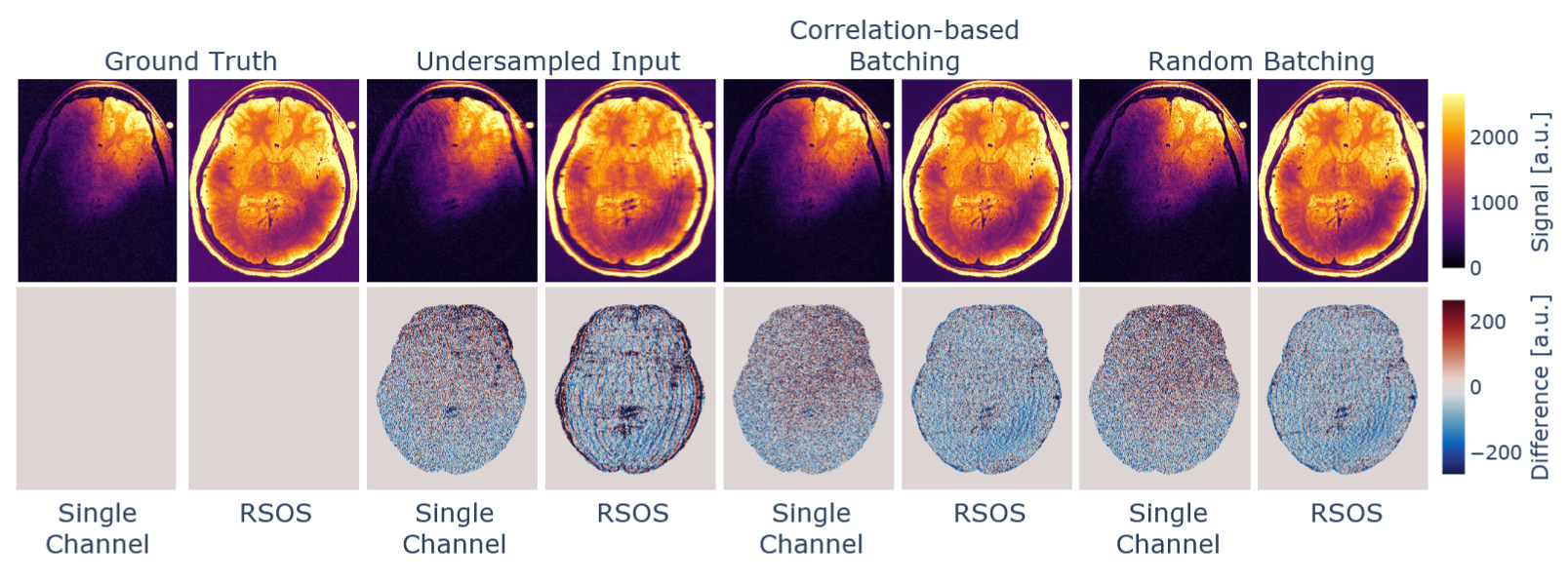
To evaluate the batching influence, we reconstructed retrospectively undersampled in vivo data (see data & hardware section), varying the used channel-batching method. The data was jointly reconstructed per batch across the channel-batches and the number of available contrasts. This procedure was done per-slice, as the channel correlations are dependent on the coil sensitivity profiles, which will vary across the extent of the input volume.

The data \(\boldsymbol{Q} \in \mathbb{C}^{N_x \times N_y \times N_s \times N_c \times N_e}\) was reconstructed slice wise for the \(N_s = 15\) slices. For each slice we combined batches of \(n_{bc} = 4\) channels and all echoes, purposely choosing a low cluster size to evaluate the influence of the clustering. Hence, the input data contained of the matrices \(\boldsymbol{Q}_i \in \mathbb{C}^{N_b \times N_x \times N_y \times N_n}\), where \(N_b = N_c / 4\) and \(N_n = 4\ N_e\).

The algorithm was set up using a rank parameter \(r = 120\) and the neighbourhood patch side-length was \(p_s = 5\). We proceeded with two different reconstruction strategies, which differed only in the preparation of the data batches, while all other reconstruction parameters remained constant. That is, (a) the channel dimension was split in chunks of size 4 to form \(\boldsymbol{Q}_i\) from the input data stream, and (b) the input data was subject to the channel-correlation-based batching with cluster size 4. This led to different channel combinations per slice.

The aim of this experiment was to evaluate the influence of mutual information across a batch. We hypothesised that using channels with a higher cross-correlation would yield increased low-rank matrix properties and thus possibly increased LORAKS performance, which would also support the use of coil compression techniques.

Data scaling and fast SVD methods

In addition to batching or compression strategies, other implementation details can be changed to accomodate increasing matrix sizes inherent in high-resolution joint-reconstruction MRI settings. Specifically, the computational performance of the matrix decomposition at the core of the low-rank enforcement is poor if SVD is employed. Since SVD is a heavily used technique in many data-driven sciences, performant variations have previously been suggested.¹⁷ Besides using the built-in torch.svd_lowrank method (LR-SVD)²⁶ which mirrors computational gains described in prior work,²⁵ we implemented matrix decomposition methods in PyLORAKS to increase computational performance. Since randomised variants of SVD do not specifically leverage or are dependent on the Hankel-like structure, and are suited for strong spectral features found in LORAKS matrices, reliable subspace capture is assumed in their deployment.⁶⁶

The following variation of methods were implemented for benchmarking as they were found computationally beneficial compared to a standard SVD: a randomised SVD (rSVD) method¹⁷ similar to LR-SVD, subspace-orbit randomised SVD (SOR-SVD),¹⁶ and a randomised QLP (RAND-QLP) algorithm.⁶⁷

All randomised matrix decomposition algorithms were previously found to benefit from using power iterations \(n_\text{iter}\) and oversampling \(o\),²⁶ two parameters facilitating the randomised sampling and compression of the input data. In the process, a data matrix of reduced size is formed to which a QR decomposition is applied, resulting in the computational benefit. This matrix is of rank \(m_r = r + o\), i.e. the complexity of randomised SVD variants scales with the target rank \(m_r\), which is usually much smaller than the input matrix size (\(\min(m_x, m_b)\)) for joint-reconstruction of high-resolution input. We used empirically determined values \(n_\text{iter} = 2\) and \(o = 10\) for all randomised decomposition implementations, which have been found to increase estimation accuracy.¹⁶

The matrix \(\boldsymbol{V}\) in equation 2 is estimated from the nullspace of the LORAKS operator matrix built from AC data (\(\boldsymbol{M}_{AC}\)), consequently minimising the use of matrix decomposition methods in AC-LORAKS to a single nullspace estimation. Increased computational efficiency previously was reached by using an eigenvalue decomposition on a Hermitian matrix \(\boldsymbol{A} = \boldsymbol{Q}\ \text{diag}(\boldsymbol{\Lambda})\boldsymbol{Q}^{\boldsymbol{H}} \in \mathbb{C}^{m_b \times m_b},\ \Lambda \in \mathcal{R}^{m_b}\), built from \(\boldsymbol{A} = \boldsymbol{M}_{ac}^{\boldsymbol{H}}\boldsymbol{M}_{ac}\), reducing the dimensionality to the shorter axis (usually \(m_b\)). The nullspace can be estimated using the trailing \(m_b - r\) vectors \(\boldsymbol{Q}[r:]\) of the eigenspace corresponding to the lowest eigenvalues. Thus, we included PyTorch torch.linalg.eigh function (EIGH) in the investigation of rank-revealing methods, as its Matlab counterpart was found to perform best in the M-LORAKS default implementation. An algorithm for randomised nullspace approximation was also tested (RAND-NS) estimating the trailing \(m_b - r\) eigenvectors through randomised projections.²⁹

First, we evaluated the speed and memory performance of the randomised matrix decomposition methods for our large matrix sizes. This was deemed necessary as the underlying computational libraries used for matrix algebra possibly switch to different backends dependent on the matrix input sizes.⁶⁸ Thus, randomised SVD variants might not perform close to their theoretically projected memory and time complexity. We used synthetic matrices (see data & hardware section) to benchmark the matrix decomposition. Theoretical predictions about the computational complexity scaling in time and memory are available.^16,17 For an instructive overview, Figure 5 shows the complexities reached in our settings.

Second, we compared the reconstruction performance of the PyLORAKS algorithm substituting the rank-revealing operation at its core. This reconstruction was done using retrospectively undersampled in vivo data (see data & hardware section). For this experiment only the methods LR-SVD, rSVD, and SOR-SVD were used, as faster computation times and lower memory footprints were found in the above benchmark.

We used these variants for the estimation of \(\boldsymbol{V}\) in equation 2, and later approximation of the low-rank loss. For all randomised variants tested, we used a target rank \(m_r = 4\ r\), with \(r\) being the rank parameter of the PyLORAKS algorithm. We ensured the target to be much smaller than the matrix size of the LORAKS matrix (\(m_r \ll \min\{m_x, m_b\}\)), as this defines the respective method’s computational efficiency. We picked the trailing \(n_\text{eig} = m_r - r\) eigenvectors to approximate the nullspace \(\boldsymbol{V}\).

Both of these benchmark experiments were solely done using the GPU capability.

New advances and possibilities for MRI

Our target was a computationally efficient LORAKS implementation considering memory and time constraints. Thus, additionally to the presented methods, PyLORAKS can be used as drop in replacement of the current M-LORAKS implementation to offer large computational boosts. For example, the computationally demanding A-LORAKS-CS²⁴ or the OEDIPUS⁶⁹ framework can benefit from efficient and fast LORAKS computations. Furthermore, the capability of backpropagation through the algorithm makes PyLORAKS a suitable candidate to be used in physics-informed deep learning^42,43 or generative AI models,⁴⁴ separating our implementation from previous attempts to algorithm computation feasibility enhancement,^38,39 enabling new features.

To demonstrate the capabilities of PyLORAKS, we used it for a multi-echo 2D acquisition. We evaluated the choice of algorithm parameters \(r\) and \(\lambda\) on reconstruction quality, as well as for the design of an optimised sampling pattern. The presented methods generalise to arbitrary acquisition schemes.

Parameter selection

Usually, the value of the algorithm parameters \(r\) and \(\lambda\) are manually chosen by the user, and its influence is assessed empirically after reconstruction.^14,20,21 In conjunction with J-LORAKS this procedure is impractical due to low computation speed and high memory demand.

The LORAKS algorithm enforces the LORAKS operator matrix to be of rank \(r\). A low-rank parameter \(r\) encourages effective filling of missing data and denoising by reducing the variance of the available data based on the used LORAKS operator, but can introduce bias if too low rank enforcement is used.³ While the denoising capabilities of LORAKS have been demonstrated,^3,13,15 no head-to-head comparison for LORAKS denoising capabilities compared to dedicated denoising algorithms is available. However, recent studies suggest that for optimal control and results of image denoising, dedicated algorithms should be preferred.^21,63,70

On the other hand, high rank favours greater data fidelity but may fail to exploit the low-rank prior, which comes at the cost of acquisition acceleration capability. Other effects on the algorithm are more intricate. For example, in AC-LORAKS a higher rank parameter reduces the size of \(\boldsymbol{V}\) extracted from the nullspace of the LORAKS matrix used in equation 2, and thus reduces the computational cost after extraction of \(\boldsymbol{V}\).

Similar effects can be seen with changes in the regularisation parameter \(\lambda\). If the data signal-to-noise ratio is sufficient, \(\lambda\) can be set very low, which was found to be beneficial for interpolation of missing data without modifying acquired samples.¹³ Alternatively, in the true data consistency formulation \(\lambda = 0.0\) of the algorithm, the LORAKS constraint is calculated for missing data points only. This is preferable for computational reasons, as the computation iterations are only done over a reduced subset of the overall k-space.

Automation of the LORAKS parameter choices has been proposed using SURE and a soft-thresholding approach⁷¹ in conjunction with compressed-sensing and total variation constraints,²⁴ at the cost of additional computational overhead. SURE allows calculating the mean squared error in estimating a true signal from measurements corrupted by additive Gaussian noise²² using only acquired samples. Consequently, SURE has been used in the context of denoising algorithms,⁷² and was extended to reconstruction algorithms when the constraint formalism resembles linear denoising operators,⁷³ for which analytic expressions have been proposed.²³ This is possible for the independent LORAKS constraint²⁴ (\(J_r(\boldsymbol{P}({\boldsymbol{k}}))\) in equation 1).

However, the full LORAKS implementation involving data consistency and constraint regularisation (via \(\lambda\)) is nonlinear, typically necessitating Monte Carlo or Hutchinson methods to estimate the operator divergence further adding computational complexity. Furthermore, finding more complex dependencies (e.g. LORAKS rank dependence on matrix size or sampling pattern) might not be possible using SURE, as e.g. divergence with respect to a sampling pattern is not reasonably defined. Nonetheless, we included a comparison with a SURE optimised rank \(r_{\text{SURE}}\) using a method similar to Ilicak, Saritas, and Çukur,²⁴ briefly described in the supplementary material. For this other parameters (complementary subsampling scheme, number of contrasts and \(\lambda = 0\)) were kept fixed and were evaluated by the method below.

It is common for MRI studies that the data sampling method and the basic data structure (dimensionality, FOV) remain similar between acquisitions. An optimisation of the algorithm parameters and evaluation of their dependencies can be tied to the specific acquisition and is a possible prior to reconstruction of individual data acquisitions. We evaluated the reconstruction performance with respect to the algorithm parameter settings of \(r\) and \(\lambda\).

We used a fully sampled and retrospectively subsampled in vivo dataset obtained from the multi-echo spin-echo (MESE) acquisitions (see data & hardware section). The PyLORAKS joint-reconstruction was followed by a root-sum-of-squares (RSOS) channel combination to obtain magnitude data.

Since the autograd framework is not suited for mixed integer optimisation, we chose a Bayesian sampling optimisation method⁷⁴ within the wandb framework⁷⁵ (version 0.17.3). Thus, the presented parameter investigation is enabled by the computational gains of PyLORAKS. To vary the neighbourhood matrix size \(m_b\) of our input data, we varied the channel batch size \(n_{bc}\). In our optimisation, the reconstruction time for one optimisation run, for a single slice of the input data (\(304 \times 237 \times 32 \times 8\)), and joint-reconstruction took \(\sim 5\) s on average. It is varying with the choice of \(m_b\).

We introduce an overall minimisation score to optimise the input parameters \(r\) and \(\lambda\) with respect to all of our metrics, scaling each of the individual metric values accordingly:

\[\min_{r, \lambda}\ \eta_{\text{loss}} = -\eta_\text{ssim} - 0.01\ \eta_\text{psnr} + \eta_\text{nmse}\tag{7}\]

The evaluation followed three distinct aims with respect to the algorithm input parameters \(r\) and \(\lambda\):

1. Find correlations between the number of missing points and the parameters.

2. Find correlations between the used input matrix dimensions and the parameters.

3. Evaluate the influence of the undersampling pattern with respect to variation in the parameters.

This assessment is specific to the used sequence and hardware due to the available number of channels and contrasts in the joint-echo reconstruction, the individual contrast content, and SNR. Nevertheless, a number of general conclusions can be drawn from the optimisation procedure.

Sampling optimisation

PyTorch’s autograd framework, described in the loss estimation and automatic differentiation section, allows direct gradient computation via backpropagation, with additional support for complex valued differentiation using Wirtinger calculus,^76,77 essentially tracking gradients in each computation step and applying the chain rule. Further information can be found in.⁴⁰ This feature was used to inform the sampling density of the input data using a single forward and backward pass of the reconstruction algorithm. We used fully sampled data, assuming true data consistency (i.e. only computing the LORAKS regularisation part in equation 1), to compute the gradient of the PyLORAKS loss function with respect to each sampled point.

We denote the loss function in Equation 1 with \(\mathcal{L}(k)\) and compute the gradient with respect to the input by propagating through the loss objective in a single pass, obtaining PyTorch gradients attached to the k-space candidate: \[ g(x, y, c, e) = \nabla_k \mathcal{L}(k) \in \mathbb{C}^{N_x \times N_y \times N_c \times N_e}\tag{8}\] Taking \(k \sim k_{\text{true}}\) by considering a fully sampled k-space input, we note that \(\nabla_k \mathcal{L}(k) \sim \mathcal{L}(k + \delta e_i) - \mathcal{L}(k)\) can be obtained from the Taylor expansion around \(k\), using \(\delta e_i\) to indicate a small perturbation at point \(i\). Thus, under the assumption of smoothness and linearity in local k-space subregions, the gradient amplitude can be regarded as a first order predictor of the change induced by corrupting (or removing) sample \(i\). Hence, equation 8 serves as a local sensitivity measure of the reconstruction loss to each sample under the imposed low-rank constraint.

We interpret a larger \(\lvert g \rvert\) as a sign of greater importance of the respective samples to the image reconstruction problem. Collapsing over channels yields: \[ s(x, y, e) = \sum_{c=1}^{N_c} \bigl|g(x,y,c,e)\bigr|\tag{9}\] This way we can deduce a sampling density mask across the input slice. Since in our case, we were interested in subsampling along the phase encode dimension of a 2D sequence, we aggregated to obtain the phase encode density per index \(i_y\) and formed a probabilistic sampling density per echo:

\[ d_e\left(i_y\right)=\sum_{k_x} s\left(k_x, i_y, e\right) \tag{10}\]

\[ w_e\left(i_y\right)=\frac{d_e\left(i_y\right)}{\sum_{k_y} d_e\left(k_y\right)} \tag{11}\]

Complementary echo sampling has previously been shown to increase the reconstruction performance of LORAKS.^13,52 Thus, we sampled a mask from \(w_e\) per echo using an adaptive sampling method⁷⁸ to ensure complementarity across echoes.

We applied this procedure to fully sampled in vivo MESE data from each participant (see data & hardware section) to compute one-pass gradients of PyLORAKS and derive an average \(w_e(i_y)\). Averaging across subjects yields a nominal density for the MESE 2D sequence. Because the gradient field is contrast- and sequence-dependent, the resulting density should be viewed as a data-driven guideline that can be recomputed for other sequences or contrasts.

The obtained sampling pattern was used for retrospective undersampling of the data and compared to the four other 2D sampling strategies given in the previous section. We used 36 AC lines and an acceleration factor of 5 with respect to the coverage outside this region. Hence, due to the data size, each echo was sampled using 76 lines.

The undersampled data was subjected to PyLORAKS joint-reconstruction using the same parameters in all reconstruction runs. The channel batch size was set to \(n_{bc} = 8\). LORAKS parameters where \(\lambda = 0.0\), i.e. true data consistency, and \(r = 150\).

The resulting reconstructions were Fourier transformed and channel-combined using an RSOS combination to obtain magnitude image data. We used the same metrics to assess the reconstruction quality: NMSE, PSNR, and SSIM.

We conducted an additional validation experiment. For each k-space point \(i\) in the fully sampled dataset, we removed the sample by inserting 0, and measured the degradation to the full k-space reconstruction, using \(\eta_{\text{NMSE}}\) (as well as \(\eta_{\text{LOSS}}\) defined in equation 7: \[ \Delta_i = \eta(k_{\text{fully sampled}}, k_{i, \text{dropped}})\tag{12}\] Effectively, we measured the k-space interpolation ability of LORAKS for each point \(i\), and we take \(\Delta\) as the ground truth for the location importance to compare against the density obtained via gradient propagation in Equation 11 by calculating Pearson and Spearman correlation coefficients.

This approach is computationally exhaustive, necessitating a full reconstruction run for each k-space point. Thus, we used some simplifications for the comparison: We adapt aggregating the readout direction and channels, as in the gradient-based optimisation method (Equation 9). Hence, we are calculating Equation 12 per phase encode, zero-filling each full line at a time.

The reconstruction was done using the same settings as above (channel batch size \(n_{bc} = 8,\ \lambda=0.0, r = 150\)) and took \(\sim 2\) h per slice iterating through all phase encode lines per echo, except for lines in the AC region as this would yield erratic AC-LORAKS performance. For comparison, the single-pass computation using propagation of Equation 8 took \(\sim 4\) s per slice.

Results

Algorithm innovations and technical implementation

Different tests and validation runs demonstrated that the implementation of PyLORAKS achieved the same reconstruction fidelity as M-LORAKS when using equal algrotihm parameters. An exemplary comparison can be found in the supplementary material.

Computational speed

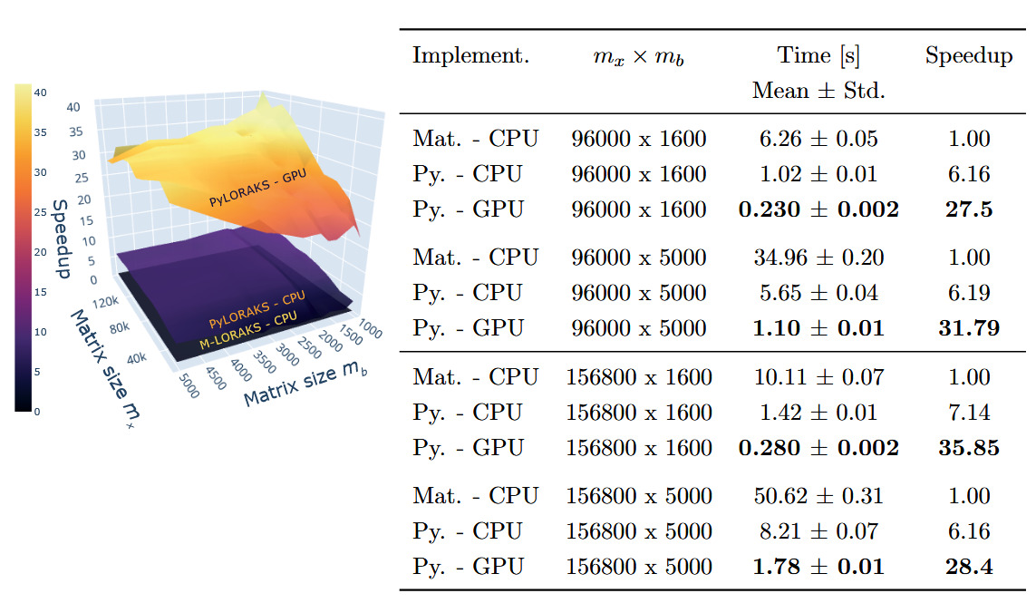
The PyLORAKS implementation offers faster computation compared to M-LORAKS. The speed differences between PyLORAKS in CPU and GPU processing modes versus the (CPU only) M-LORAKS implementation can be found in Figure 2.

Figure 2.PyLORAKS performance speed benchmarking data.

Two \(m_x\) and \(m_b\) matrix sizes, respectively, were selected from the benchmark, and the computation times are provided in the table to the right. For each matrix size, the last column gives the fraction of M-LORAKS computation time over the respective PyLORAKS computation time, which is also depicted in the plot to the left.

A great improvement was achieved using PyLORAKS compared to M-LORAKS irrespective of matrix sizes. Across all benchmarked input matrices we found an average speed increase of 5.75 using PyLORAKS and CPU computations. However, the highest speedups were observed when increasing spatial matrix size \(m_x\) and fairly small or moderate neighbourhood matrix dimension \(m_b\). This is presumably due to the improvements in linear memory layout and parallelisation of computations. The performance of the actual matrix decomposition algorithm (eigh in this case) was not assumed to vary drastically between Matlab and Python implementations and scaled with the smaller matrix dimension, i.e. \(m_b\).

The PyLORAKS GPU implementation resulted in a substantial acceleration of computations, yielding an average speed increase of 29.11 across all tested matrix sizes compared to M-LORAKS. Note that due to the high computational demands, LORAKS is commonly used on a per-slice computation iteration (in M-LORAKS and PyLORAKS). Hence, the per-slice time savings presented here additionally scale with the number of slices to process, considering whole volume reconstruction. The resulting speed improvements mark a step towards real-time-imaging applicability of joint-reconstruction PyLORAKS, with the computational speed well below 1s for scan sizes encountered in high-resolution imaging (see Table 2).

Furthermore, the matrix sizes are given by \(m_x \sim 2 \times N_x \times N_y\) and \(m_b = 2 \times N_c \times N_e \times N_b\). The biggest matrix sizes given in Table 2 correspond roughly to a data size (without slice dimension) of \(280 \times 280 \times 32 \times 3\), i.e. a scan using a 32-channel receive coil and three contrasts, or similar configurations if batching is used.

Memory

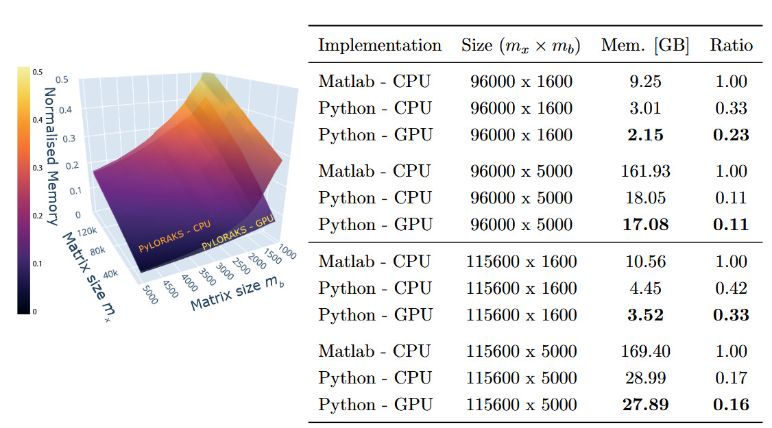
The memory allocation of the algorithm was tracked, including the data loading to RAM and the overhead created by the software (e.g. memory allocation for matrix decomposition operations). The resulting benchmark is visualised, and a subset of the numbers are given in Figure 3. The projected memory complexities match literature values.^16,17

Figure 3.PyLORAKS performance memory benchmarking data.

Two \(m_x\) and \(m_b\) matrix sizes, respectively, were selected from the benchmark, and the profiled memory is provided in the table to the right. For each matrix size, the last column gives the fraction of PyLORAKS memory footprint over the respective memory used by M-LORAKS, which is also depicted for the plot to the left. Compared to M-LORAKS, the highest memory savings were be achieved with relatively small spatial dimensions \(m_x\) and large neighbourhood dimensions \(m_b\). We randomly tested for variability in the estimates for a small subsample of the data but found no significant changes (\(std < 0.01%\)).

Averaged across all tested matrix sizes, we found PyLORAKS to be using only \(21.2 \%\) of the memory compared to M-LORAKS for the same computation when using CPU processing. This is presumably due to increases in efficiency of memory allocations and linear indexing and the absence of any loops in the core functionality. The memory usage ratio compared to M-LORAKS dropped even more for big matrix sizes, to as low as \(11 \%\) in some cases, as can be seen in Figure 3.

In both cases modern hardware might be able to efficiently use parallel CPU computing to process datasets. However, our memory tracking was set up to follow all child processes created by the algorithms. Thus, if hardware memory is limited, the processing might not be done in parallel but sequentially and is possible with smaller available total memory than the values presented here, at the cost of increased computation time.

For the PyLORAKS GPU computation mode an even smaller memory footprint was achieved, using only \(16.4 \%\) compared to the M-LORAKS processing when averaged across all tested matrix sizes. Again, the memory usage ratio compared to M-LORAKS was lower for big matrix sizes, reaching below \(11 \%\) in some cases, as can be seen in Figure 3. The drop compared to the PyLORAKS CPU mode is due to careful transfer of only necessary data to the GPU RAM, which on average saves around \(1\ \text{GB}\) of memory. However, it follows that PyLORAKS GPU mode allocates this amount of memory additionally on CPU memory, primarily for loading in the data.

Note, AC-LORAKS is based on an approximation of \(\boldsymbol{V}\), which decreases in size with increasing rank. This way, the allocated memory is not only dependent on the input data size but also the algorithm parameters (\(r\) and \(\lambda\)).

Data combination and batching

The reconstruction of the data using different channel combination methods in conjunction with batching along the channels can be seen in Figure 4. We compared the reconstruction to the fully sampled data after brain masking, and the derived metrics can be found in Table 1. The channel-correlation-based batching resulted in increased performance metrics, while the difference in the reconstruction is hard to notice visually. This can be regarded as a minor performance boost but likely will not suffice, e.g., to be traded for higher acceleration in the acquisition process.

Figure 4.Reconstruction performance using different channel batching strategies for limited memory in joint-reconstruction.

In the first row, we show magnitude data for each reconstruction with one randomly selected channel and the RSOS combination of all channels per column respectively. As ground truth data, we used a fully sampled data set (first two columns), which was retrospectively undersampled (second and third columns). The bottom row shows the difference of the fourier transformed output to the ground truth data. Similar reconstruction results can be achieved for random batching of channels (two rightmost columns) and the proposed channel-correlation-based method (fifth and sixth columns), with incrementally reduced difference to ground truth visible for the latter.

Data scaling and fast SVD methods

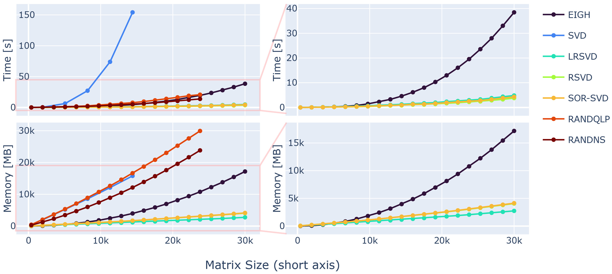
For optimisation of the loss function in 1, the rank-revealing decomposition (SVD or eigenvalue decomposition) can be substituted by a randomised variant more effective for big matrix sizes. The performance of each method was tested separately, processing the decomposition on simple input matrices. The speedup of the respective method was substantial and can be appreciated in Figure 5. For growing matrix sizes, an SVD scales linearly in Memory usage and quadratically in computation time.

Figure 5.SVD variant benchmark.

Computation time (top row) and maximum allocated memory (bottom row) are given for different rank-revealing matrix decompositions using random input matrices with various sizes. The standard SVD algorithm performs poorly with respect to computation time, showing a \(O(m_b) \sim m_b^3\) complexity with respect to the input. Additionally, the memory consumption scales linearly with the input size. While other variants showed much increased computation times, the RANDQLP and RANDNS algorithms also show comparable memory consumption. The inset on the left column focused on variants with increased computation times and much lower memory consumption (EIGH, rSVD, SOR-SVD), zoomed in on the right column. For increasing matrix dimensions, it is clear that the EIGH algorithm is outperformed by the randomised variants.

The memory overhead of randomised versions is dependent on the target rank \(m_r\) and an oversampling parameter \(o\), making memory saving possible, as the memory allocation overhead of randomised SVD variants is dependent on the chosen target rank. Hence, memory allocation of the respective randomised methods is possible in a controlled manner, e.g. tailored to the available hardware.

While the EIGH does offer considerable performance increase (\(\sim 17 \times\) faster) compared to the standard SVD, it falls short compared to other randomised rank-revealing decomposition alternatives (see 5, right column). While the RAND-NS and RAND-QLP methods offer considerable speedup, close to what can be achieved with the EIGH method, their demand on memory is similarly high as standard SVD methods.

Further speed increases are possible by using the proposed rSVD,¹⁷ LR-SVD²⁶ or SOR-SVD¹⁶ methods, offering a \(\sim 4\)-fold speed increase for the biggest matrix dimension used in the test comparison to EIGH. The computational efficiency is projected to be even greater with higher-dimensional input. Thus, the use of randomised SVD variants is preferable, especially with increasing matrix sizes encountered in high-resolution MRI reconstructions.

Similarly, EIGH, rSVD, LR-SVD and SOR-SVD are all preferable in terms of memory consumption. Where again the former shows deficits, with more than \(3\)-fold more memory demand for big input matrices. The memory consumption agrees well with complexity estimates given in literature.^16,17

Figure 6.SVD variant reconstruction performance.

A fully sampled dataset was used as ground truth (first column). Data is shown for two randomly selected channels (first two rows) and the RSOS channel combination (third row). The difference of the channel combined magnitude image to the ground truth is given in the bottom row. Retrospective under-sampling (second column) was used and subject to PyLORAKS reconstruction using different rank-revealing decompositions (respective following columns). The result appears similar in all reconstructions and close to the ground truth. The LR-SVD (4^th column) shows the lowest error.

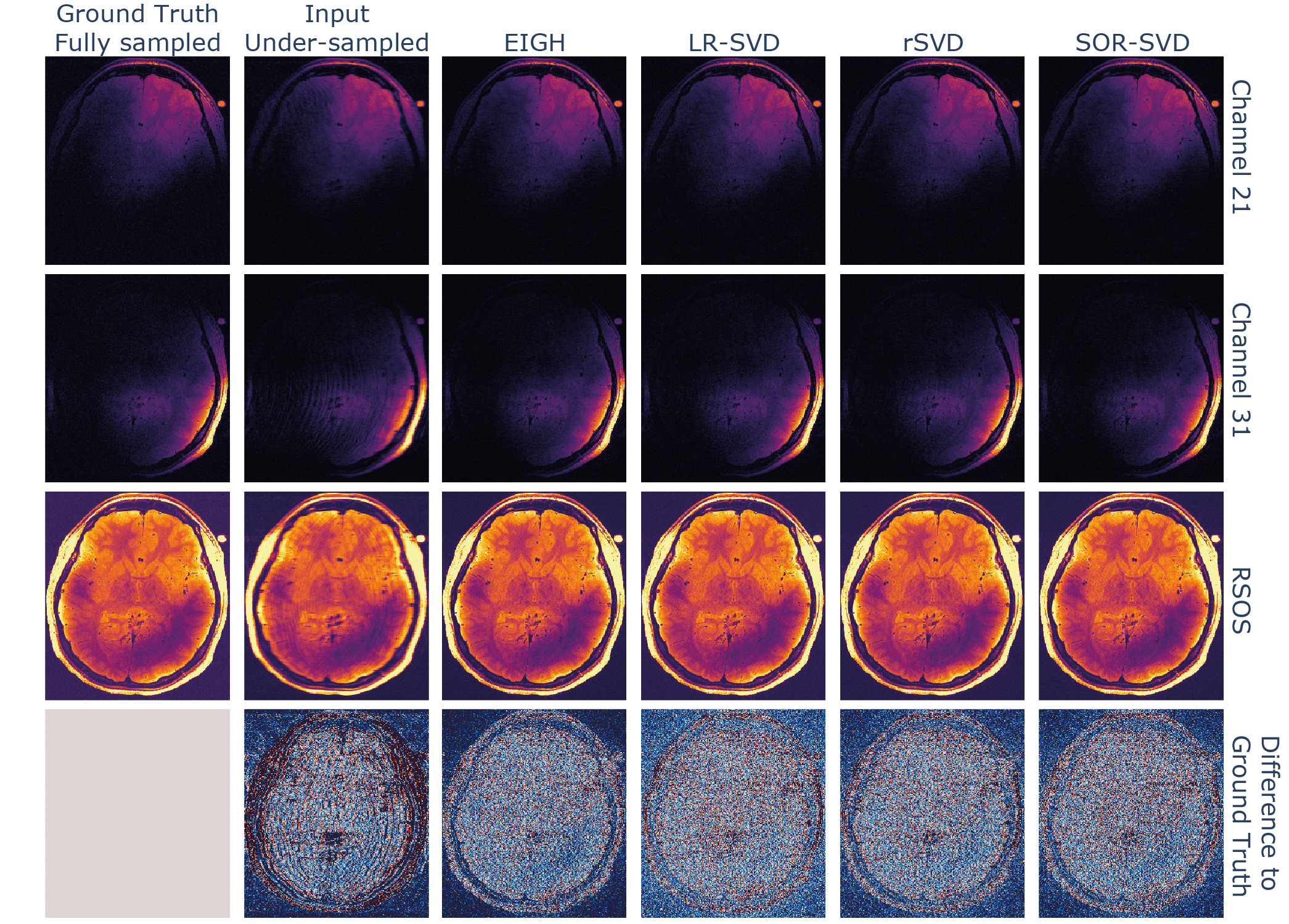
We compared the reconstruction performance of the SVD variants with favorable memory and time demands, which is shown in Figure 6, by substituting the matrix decomposition operation within the algorithm with the respective method. All tested randomised SVD variants showed similar reconstruction performance to the EIGH (default in M-LORAKS) method, the used metrics are shown in Table 2. While the LR-SVD method appears to be optimal with respect to the NMSE and PSNR, the original EIGH method achieves the highest SSIM score. However, rSVD and SOR-SVD were able to achieve \(\sim 5 - 7 \%\) quicker computations for the dataset used.

A substitution of the rank-revealing operation when using LORAKS reconstruction for high-dimensional input data was beneficial computationally and resulted in comparable image quality as the standard LORAKS reconstruction implementation. The computational benefit of using randomised SVD variants is dependent on the number of nullspace eigenvectors used for the nullspace approximation (here \(n_\text{eig} = 3 r\)), as well as the matrix sizes in general. Presumably, even higher speedup is possible given the randomised SVD benchmarks in Figure 5 when bigger matrix sizes are involved or with optimising the dimensionality used for nullspace approximation.

New advances and possibilities for MRI

The results of the acquisition optimisation for our MESE sequence are presented in the following, using different features of the PyLORAKS framework, such as its backpropagation capabilities.

Parameter selection

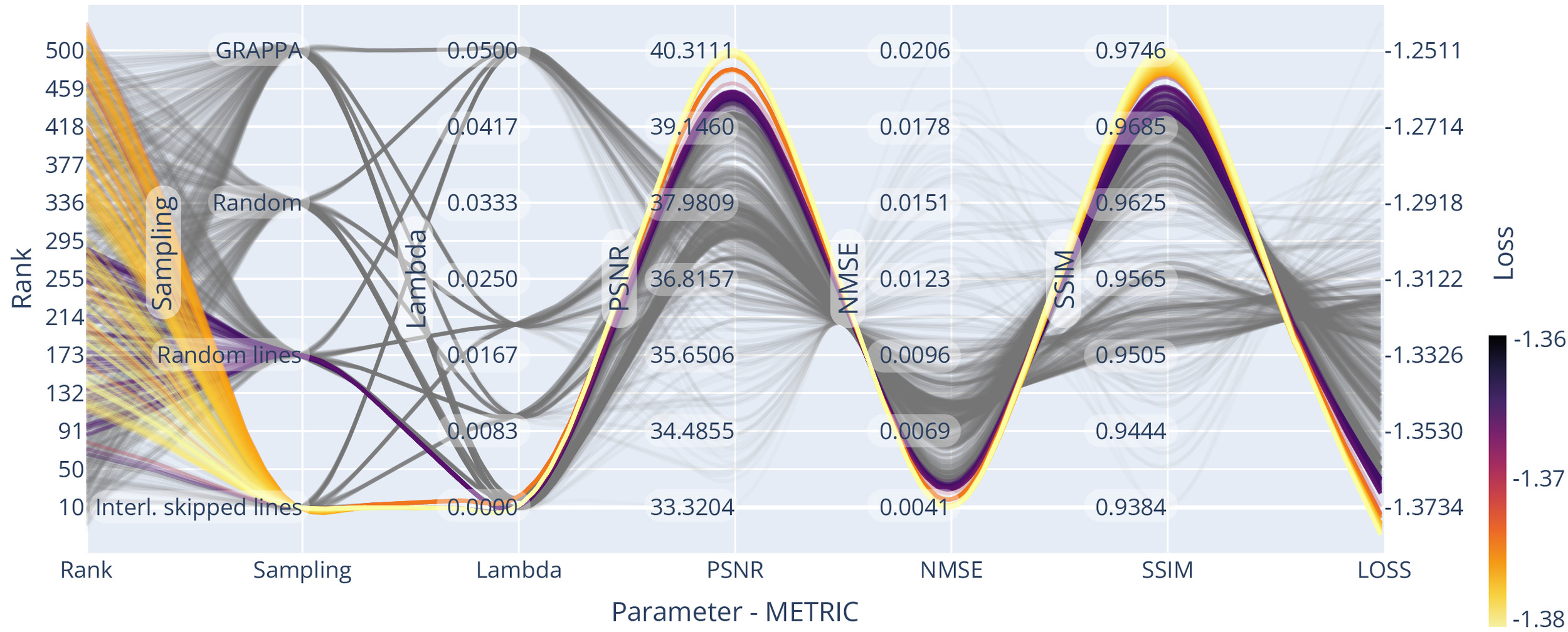
We optimised the reconstruction algorithm parameters for the highest quality reconstruction of our data compared to a fully sampled dataset. We obtained parameter trend-lines for \(r\), \(\lambda\) and the used sampling patterns for a 3-fold acceleration, which can be seen in Figure 7. Less heterogeneous k-space coverage across the sampling pattern for joint contrasts, like in GRAPPA, reduced the resulting reconstruction quality. Using random-line sampling or interleaved skipping of outer k-space lines across different contrasts yielded the lowest loss values, which is in line with previous findings of performance increases with complementary echo sampling.^13,52

Figure 7.Parameter optimisation trendlines.

The three varied input parameters are given on the left (Rank, Sampling, and Lambda) and their influence is plotted against the three evaluation metrics PSNR, NMSE and SSIM, and a combined overall loss score given in equation 7. Randomised lines and interleaved skipping of outer lines per echo resulted in higher scores compared to grappa or random sampling. For all sampling methods, the true data consistency formulation (\(\lambda= 0.0)\)) provides optimality. The rank parameter values vary between 120 and 200 and, dependent on the used sampling scheme, are optimal at 143 for the interleaved line sampling.

We found optimality in all metrics using the true data consistency formulation (\(\lambda = 0.0\)) over the regularised version, updating only missing data points in the reconstruction. Whenever noise suppression and handling of imperfect data was not one of the main aims in the reconstruction or could be achieved with dedicated processing steps, the true data consistency formulation offers advantages.

For example, for all considered sampling patterns except GRAPPA, setting \(\lambda = 0.0\) resulted in the highest SSIM and PSNR and the lowest NMSE. On average the NMSE increased \(\geq 10\%\) for \(\lambda = 0.001\) compared to \(\lambda = 0.0\) and much higher values for higher settings of \(\lambda\). Similarly, SSIM decreased \(1 - 2 \%\) for \(\lambda = 0.001\) compared to \(\lambda = 0.0\), and again even lower values were found for higher settings of \(\lambda\). For the GRAPPA sampling, low values of \(\lambda = 1e-3\) resulted in loss minimisation and a small advantage over the true data consistency setting, which corresponds to other findings¹³ for GRAPPA acquisitions.

However, GRAPPA sampling was found to underperform compared to other sampling methods, possibly due to the lack of complementary sampling across echoes. For example, the NMSE was \(\eta_\text{nmse} = 0.0077\) and SSIM was \(\eta_\text{ssim} = 0.955\) for GRAPPA sampling (\(\lambda = 1e-3\)), compared to \(\eta_\text{nmse} = 0.0049\) and \(\eta_\text{ssim} = 0.972\) for echo - interleaved skipped line sampling (\(\lambda = 0.0\)).

The Bayesian optimisation framework was arriving at (or approximated) the optimum already after few iterations (\(\sim 15\)). Thus finding a close to optimal rank parameter for a single slice was possible in \(\sim\) 75 s, totalling \(\sim\) 35 m for the full volume. We included trendlines from a more exhaustive search for visualisation purposes in Figure 7, Figure 9 and Figure 10 to spot trends more easily.

Optimal rank parameters for all subsampling schemes were in similar ranges (\(120 - 200\)). The optimal loss for joint-reconstruction of our input (slice dimensions \(304 \times 237 \times 32 \times 8\) with batched channels) was found using echo - interleaved skipping of lines \(\lambda = 0.0\) and the rank \(r = 143\). For comparison, we used the SURE optimisation approach (see the supplementary material) on AC data of the same input, yielding an optimal rank value of \(r_{\text{SURE}} = 141\).

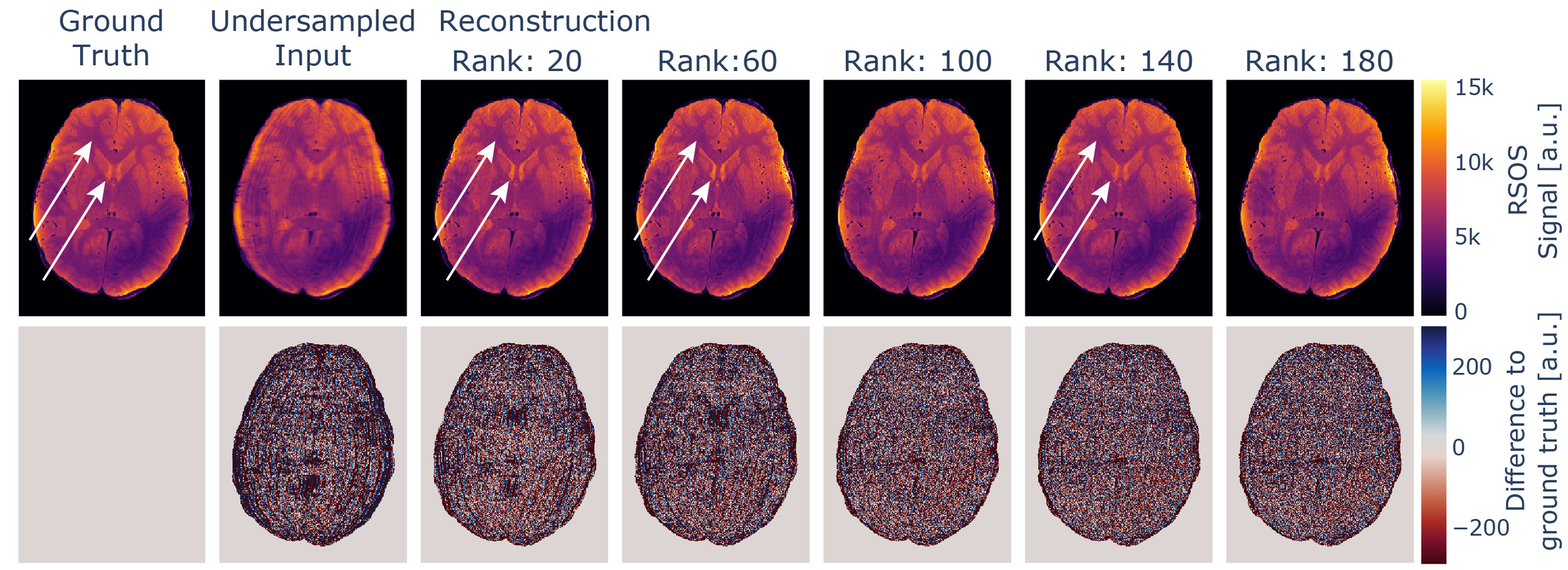
If the rank parameter is selected to be too low, the increase in the loss is accompanied by intensity variations in the reconstructed images not immediately evident if no ground truth for comparison is available. If further processing involves physical modelling of the data, as e.g., in our case the estimation of quantitative \(R_2\) values, this will degrade the robustness of the estimates. This influence is depicted in Figure 8 and is presumably caused by mixing of contrasts, as for MESE data, late echoes show a higher dynamic range between white matter and ventricles compared to early echoes, which is visible in the data. The effect might be more subtle and might not disappear the same way as e.g. aliasing artefacts with increased rank settings.

Figure 8.Influence of rank parameter on joint-reconstruction.

RSOS channel combinations are shown in the upper row, with the fully sampled data as a reference (first column), and undersampled input shown in the second column. The second row provides the difference to the fully sampled ground truth data. Using a small rank parameter (e.g., third and fourth column) has intricate effects. Residual aliasing is visible, reducing in severity with increasing rank parameter. Additionally, a brighter, delineated ventricle is visible (white arrow) together with slightly reduced intensity, for example, in parts of white matter (white arrow). This is in line with contrast mixing across echo times, considering transverse decay in MESE data causes high signal contributions from CSF or water contributions and lower contributions elsewhere.

All evaluated metrics, however, approach an asymptotic value below the respective optimum with increasing rank parameter. Thus, using a higher rank parameter does not affect the reconstructed image in the same way. With increasing rank parameter the reconstructed image appears to be more granular, but intensity variation artefacts were absent, as also visible in Figure 8. Thus, we recommend using rather high rank parameter settings.

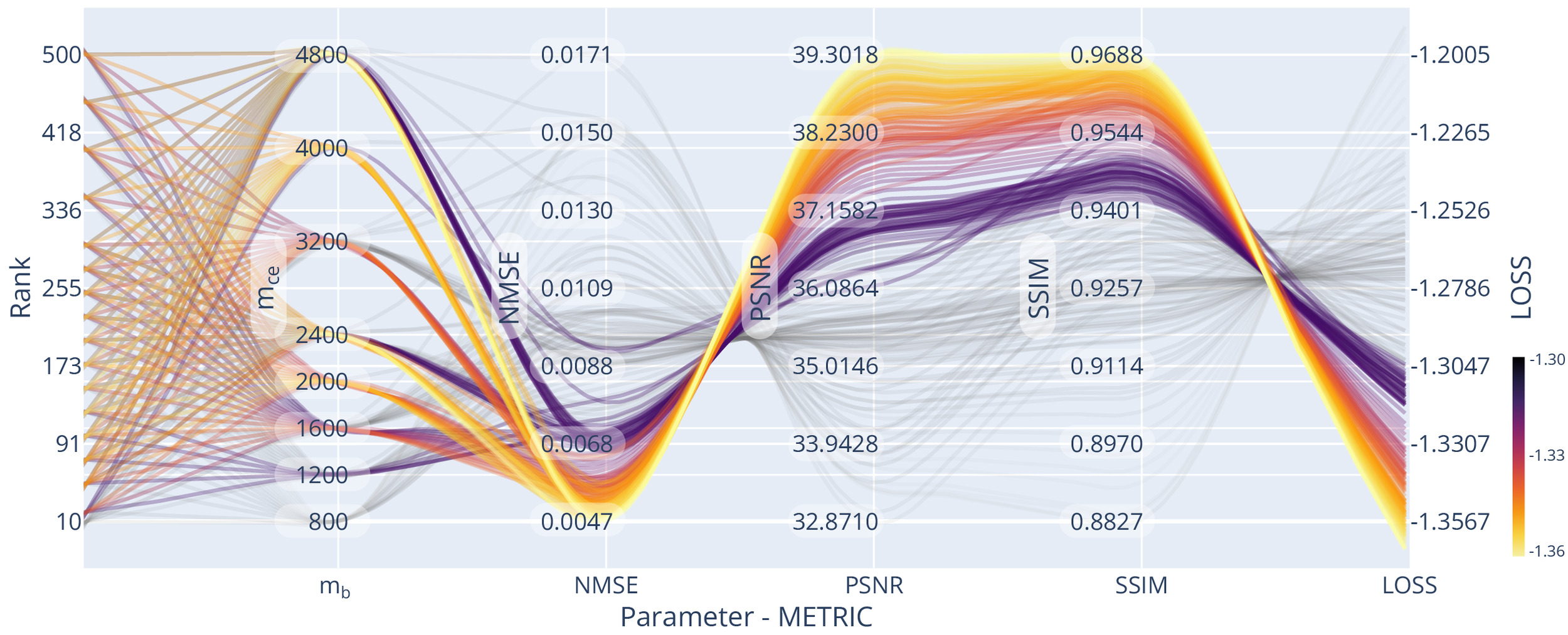
We evaluated the influence of rank, matrix size, and acceleration on reconstruction quality, using the previously found optimal settings regarding the subsampling pattern and \(\lambda = 0.0\). The trendlines can be seen in Figure 9. The joint-reconstruction of as many channels and echoes as possible (i.e. high \(m_b\)) improves reconstruction quality.

Figure 9.Parameter optimisation trendlines for varying the algorithm rank parameter and input data matrix size (Rank and \(m_b\)).

The influence on the three evaluation metrics PSNR, NMSE, and SSIM is plotted and optimisation with respect to a combined loss given in Equation 7. Optimal rank varies with input matrix size. The minimisation of loss correlates with an increase in matrix size, i.e., joint-reconstruction with the maximum number of input channels and contrasts results in increased scores in the evaluated metrics.

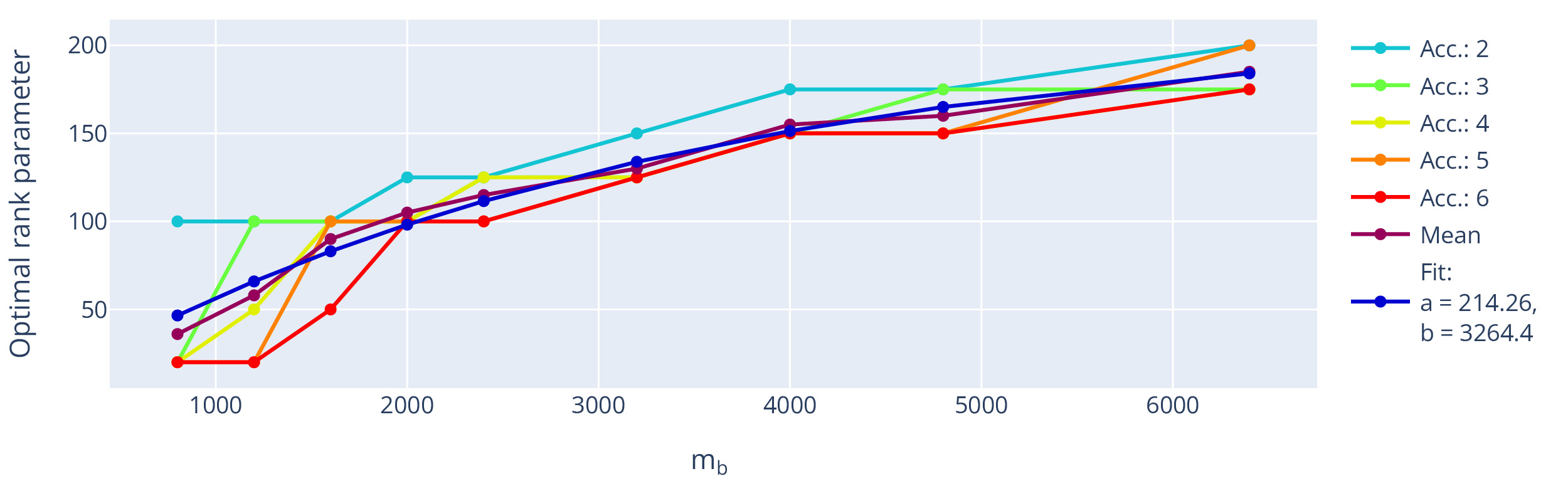
The extracted optimal rank using this setting (fixed sampling and using true data consistency) is shown with respect to the number of missing k-space points, i.e. the acceleration, in Figure 10. The optimal rank is dependent on the matrix size \(m_b\) but shows little influence on the used acceleration. Assuming the information found in local k-space neighbourhoods is limited, we expect asymptote of the optimal rank parameter.

Figure 10.The optimal rank is shown against the short matrix size \(m_b\) of the LORAKS matrix.

The spatial dimension \(m_x\) was kept fixed, as was the sampling scheme (echo interleaved skipping of lines) and the \(\lambda= 0.0\) parameter. For this setting the optimal rank parameter was obtained by Bayesian optimisation sampling. This optimal rank setting slightly varies with the used acceleration, i.e., the amount of missing data in the matrix, where generally higher rank parameter achieved reconstruction optimality with lower acceleration factors. However, the general trend shows asymptotic behaviour of the optimal rank driven primarily with the matrix size \(m_b\) rather independent of the acceleration used, approaching a value around 200 for big matrix sizes.

Fitting an exemplary asymptotic function modelling the trend, e.g., \[f(x) = a (1 - e^{-x/b}),\tag{13}\] to the mean value across used accelerations, the rank parameter would thus approach an optimum at around 214 for big input matrices, which is close to the default settings used in the original multichannel M-LORAKS algorithm.¹⁸

If a fully sampled dataset or subset is available or can be acquired for piloting a particular sequence acquisition scheme, the PyLORAKS framework includes the presented optimisation procedures for finding suitable algorithm settings using Bayesian parameter optimisations.⁷⁴

Sampling Optimisation

The automated gradient computation through the PyLORAKS algorithm was used for estimation of the sampling densities \(w_e\), which are shown in Figure 11.

Figure 11.Results of validation experiments.

The first row shows the results of the validation experiments, after extracting \(\Delta_i\) per phase encode, \(η_nmse\) and \(η_loss\) were calculated, yielding a sensitivity measure of reconstruction fidelity reduction dependent on phase encode position \(i\). Computation of the Person correlation coefficient (top left) and Spearman correlation coefficient (top right) between \(\Delta_i\) and \(w_e\) is shown yielding high correlation between individual echo sensitivity measures. The sampling density per echo \(w_e(i_y)\) (Equation 11) is obtained (bottom row), deduced after aggregation and normalisation of one-pass back-propagated gradients. Excluding the AC region, a similar pattern for all echoes is visible with an increase in sampling importance towards the k-space centre.

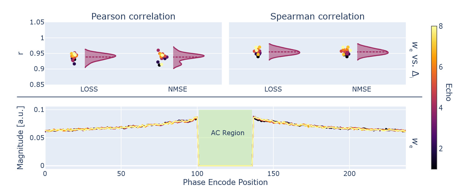
An additional validation experiment was used to find \(\Delta_i\) given in Equation 12 using ablation of each respective phase encode line. \(\Delta_i\) was computed using \(\eta_{\text{nmse}}\) and \(\eta_{\text{loss}}\) from Equation 7. These measures of sampling importance were correlated to \(w_e\) using Pearson and Spearman correlation coefficients. The individual data per echo is given in Figure 11. When using the average, across all available echoes, the following coefficients were computed: Pearson correlation \(r=0.986, p=0.0126\) and Spearman correlation \(r=0.990, p=0.0171\) for \(\Delta_i(\eta_{\text{nmse}})\) versus \(w_e\), and Pearson correlation \(r=0.981, p=0.0126\) and Spearman correlation \(r=0.991, p=0.0172\) for correlating \(\Delta_i(\eta_{\text{loss}})\) versus \(w_e\). However, a single gradient backpropagation pass through PyLORAKS was achieved in \(~ 1 / 1500\) of the computation time.

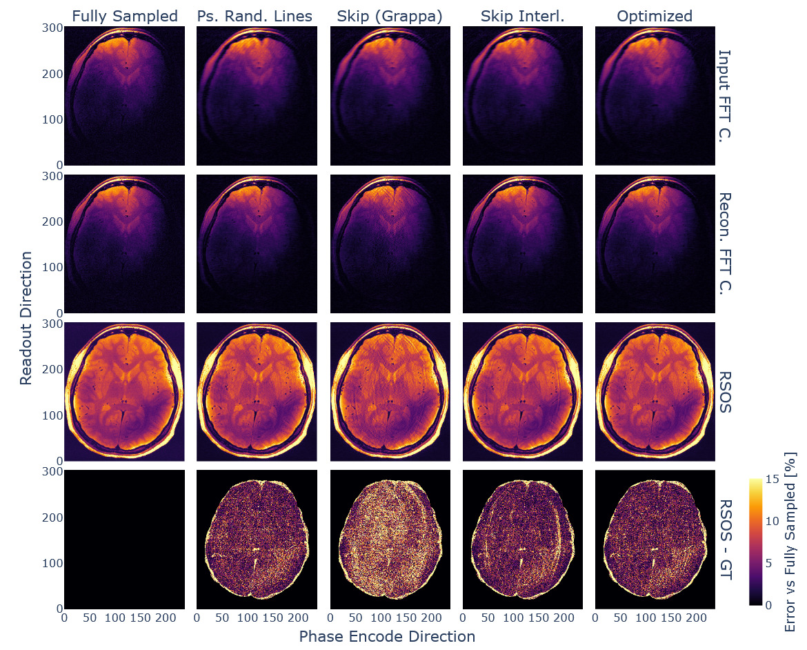
Using the obtained \(w_e\) and an adaptive sampling method⁷⁸ we created a sampling pattern matching the input dimensions, AC line, and acceleration constraints. The resulting sampling pattern, alongside the ones used for comparison, can be seen in Figure 12, showing sampling variation across echoes for the phase encode direction.

Figure 12.Tested sampling patterns to test optimal reconstruction results.

A fully sampled sampling is given in the left column. Columns 2-4 show the sampling patterns described in the sampling subsection, and the right column depicts the sampling obtained by the proposed optimisation approach. The colours are used only for easier visualisation of the individual echo samplings, black lines indicate zero-filling.

The obtained sampling pattern was tested against the other 2D joint-echo sampling strategies. The resulting reconstructions are exemplified in Figure 13. We evaluated the reconstruction performance, and the respective evaluation metrics are given in Table 3.

Figure 13.Reconstruction performance with respective input undersampling pattern.

The pattern detailed in Figure 12 was reconstructed using the same algorithm settings for PyLORAKS, and compared to the fully sampled reference given in the left column. For each input a simple FFT to image space shows the influence of the sampling pattern on aliasing artefacts in the first row for a randomly selected channel and the first echo. The second row displays the respective reconstruction after using PyLORAKS for the same channel and the first echo. We used an RSOS channel combination to obtain magnitude images of the first echo provided in the third row, of which the difference to the reference RSOS was calculated and is displayed in the fourth row.

Consequently, the optimised subsampling strategy ensured optimal reconstruction metrics, close to the previously found optimum for the interleaved line skipping method. Noticeably, the latter provided similar overall scores, but the reconstructed images showed residual aliasing artefacts. The obtained sampling density function was similar for all used in vivo datasets.

The strategy allows for data-driven optimisation of the sampling scheme for a given MRI acquisition, which in turn can facilitate enhanced reconstruction results. Alternatively, the gained reconstruction capability can be traded for increased acceleration or resolution. Furthermore, PyLORAKS reconstruction might be considered as a building block for physics-informed AI modelling, due to its capabilities for gradient propagation.⁷⁹

Discussion

In this study, we introduce PyLORAKS to address the computational demands of low-rank-based joint reconstruction for state-of-the-art MRI datasets. By incorporating efficient parallel CPU and GPU computations, PyLORAKS serves as a fast tool for reconstruction of high-resolution MRI data. Beyond speed, PyLORAKS enables scaling to high-dimensional data by replacing classical matrix decompositions with randomised variants, which will be required for future increases in data size.

We demonstrate the capabilities of our framework by presenting data-driven acquisition optimisations and showing a subsampling optimisation that improves reconstruction quality for multi-echo acquisitions, enabling higher acceleration factors. Furthermore, we present a Bayesian parameter optimisation strategy for evaluating optimal algorithmic parameters that results in increased reconstruction fidelity. We observed improved performance with true-data consistency (\(\lambda = 0\)) and note inter-contrast artefacts when the rank parameter was set too low, relative to the LORAKS matrix size. The resulting extensible framework opens up potential, specifically through the implementation of backpropagation. This enables future integration with acquisition and reconstruction optimisation or deep learning-based data modelling.

Hardware limits and speed

Despite substantial speed increases, PyLORAKS (like LORAKS in general) benefits from modern hardware. The largest gains were achieved by using GPUs. Recent high-memory GPU nodes may be unavailable or too costly for certain research settings. Additionally, benchmarks will depend on the CPU/GPU architecture and may vary across different hardware systems.

However, we present data-combination and batching strategies to enable joint reconstruction under tighter hardware constraints. Furthermore, the openly available framework includes deployment guides for HPC/cluster or cloud use, although computational speed gains may be offset by data-transfer overhead.

In any case, PyLORAKS accelerates computations for CPU units as well. Emerging sparsity-exploiting frameworks for efficient memory handling and computation⁸⁰ may further reduce computational demands in the future.

Fast SVD methods

Randomised SVD algorithms reduce memory and time for processing of large LORAKS matrices and computational demands are tailored by target rank and oversampling. Thus, explicit control of the memory footprint with respect to hardware limits is possible, but a dedicated optimisation of the influence on the reconstruction was beyond the scope of this work.

For example, introducing randomised SVD methods will be much more efficient for P-LORAKS as the LORAKS constraint is enforced with a low-rank approximation of the LORAKS matrix, allowing for big data compression within the matrix decomposition method since \(r \ll m_b\). On the other hand, with the AC-LORAKS framework presented here, the rank enforcement is done by approximating the nullspace of the LORAKS matrix formed by AC data. This nullspace is of dimensionality \(m_b - r\) and an effective compression using randomised SVD variants has little computational benefit for small \(r\). Therefore, we decided to use a different approximation of the nullspace by computing the leading \(4 r\) eigenvectors of the nullspace by the randomised SVD method. Further increase in computational efficiency might be possible by further reduction of this dimensionality, and effective memory control is possible by adjusting to the available hardware.

Scalability and 3D acquisitions

Given the computational efficiency improvements achieved with PyLORAKS, we demonstrated effective joint-reconstruction of modern high-resolution data. However, we limited the study to slice-wise reconstruction most suited for 2D sequences. While 3D sequences can be reconstructed in this fashion (e.g. by formation of a hybrid space with the Fourier-transformed readout direction taken as the iterative dimension), 3D subsampling might benefit from extending the LORAKS neighbourhood to a 3D volume as previously suggested.^3,18 However, the scaling implications are beyond what has been investigated within the scope of this study. Not only does the neighbourhood size contribute with the power of its dimensionality to the LORAKS matrix size \(m_b \propto p_s^{n_\text{dim}}\), also the larger matrix dimension \(m_x \propto \prod{N_{x,y,z}}\) scales linearly with an added dimension. This counterbalances the improvements presented in our study and might be prohibited by memory limits in a joint-reconstruction setting and high-resolution data. We suggest using the PyLORAKS framework in iterative fashion across 2D slices to achieve the presented advantages. However, further exploitation of the use of randomised matrix decomposition methods enable higher dimensional data processing, as well as future hardware advancement possibly allows for joint-LORAKS 3D reconstruction of high-resolution data using PyLORAKS.

Noise

One aspect of joint-echo reconstruction and LORAKS reconstruction in general is its effect on imaging noise not studied in the presented research. LORAKS has previously been shown to have denoising effects, which are additionally related to specific image structures.³ The resulting spatially dependent noise reduction or amplification possibly extends across contrasts in a joint-reconstruction and, to the authors’ knowledge, has not yet been thoroughly investigated. Due to the nature of randomised SVD methods, using random sampling of the LORAKS matrix to facilitate data compression, additional effects on imaging noise are likely. In our presented PyLORAKS framework focus was placed on reconstruction of individual channel and contrast data respectively, allowing for a more straight forward investigation of noise influence compared to e.g. channel compression approaches, but is left to future research efforts.

Evaluation of algorithm parameters

The presented methods for data-driven evaluation of algorithm parameters revealed joint-reconstruction pitfalls that are applicable to other data, such as the mixing of contrast information when using too aggressive rank settings. Results such as the optimality of true data consistency or specific rank parameters may not generalise to all acquisition modalities, but the presented methods can be used to tailor the algorithm parameter settings to the specific acquisition method. Furthermore, if fully sampled data can not be acquired for reference, optimisations with respect to the parameter choice are possible using a target reconstruction. The applicability of our results to other imaging data remains to be demonstrated. Nonetheless, the usage of PyLORAKS as a drop-in replacement within reconstruction optimisations like A-LORAKS-CS²⁴ to increase computational performance opens up other pathways to data-driven parameter selection beyond the presented method. However, presenting generalisable optimal LORAKS settings remains a challenging task.

Automatic differentiation and backpropagation

We demonstrate automatic gradient computation for backpropagation through the PyLORAKS algorithm, enabling input or condition optimisation. However, great efforts were previously invested into enhancing the LORAKS framework.¹⁸ The least-squares solver mechanism is a fast and efficient method, especially in conjunction with CGD approaches, and thus has been proven to be quicker than the gradient descent used with backpropagation. This is mainly due to the update rate being unknown a priori, which is the case for most machine-learning approaches using the same PyTorch mechanism. Thus, similar loss optimisation efforts in conjunction with backpropagation might be used, for example, adopting stochastic optimisation like Adam.⁸¹ Additionally, computation of an optimal or adaptive step size is part of recent AI - research^82–84 and emerging results might be applicable to the PyLORAKS framework.

Subsampling optimisations

The automatic differentiation feature was used for end-to-end optimisation of the sampling pattern of a multi-echo acquisition, which provided an increase in reconstruction quality transferable to increased acquisition acceleration. Due to the stochastic sampling approach, the optimisation for other acceleration factors is implemented quickly. We found the obtained sampling densities to be similar across participants, and thus to be valid across equal acquisitions. However, due to the limited number of subjects, generalisation to other acquisitions or changes in acquisition parameters (such as \(T_E\) or FOV) warranting re-computation need to be further analysed in future research. In principle, the automatic differentiation framework can be used to compute a deterministic mask with additional improvements beyond the scope of this work. Furthermore, the processing relied on the availability of fully sampled data for at least parts of the FOV. To circumvent this for cases where this is not available or hard to obtain, a target reconstruction can be used instead. In any case, PyLORAKS can be suitable for integration in existing sampling optimisation frameworks like OEDIPUS⁶⁹ and thus allows for a plethora of sampling optimisation options.

Assessment

We used a number of metrics for assessment of the reconstruction quality and the optimisation procedures. Each metric (NMSE, PSNR, SSIM) has specific advantages and limitations; we consider SSIM most suitable for perceptual image quality assessment. Nonetheless, the used images have a high resolution, and reduction of image content into one quantitative metric has its drawbacks. For example, the second-best sampling pattern (based on metrics) showed notable aliasing artefacts compared to others. Thus, visual inspection of the data is still necessary, should always be carried out, and future improvements in image evaluation quantification are needed.

Conclusion

We present PyLORAKS, a fast and computationally efficient implementation of the LORAKS reconstruction approach, particularly for large MRI datasets. We incorporated joint-contrast reconstruction and optimised code to achieve high computational efficiency and a speed increase of around 5–6-fold compared to the original MATLAB implementation. Additionally, GPU parallelisation further accelerates single-slice joint reconstruction by up to 30-fold. The estimated increase in computation time scales with the number of slices, drastically reducing reconstruction time of whole volume multichannel multi-contrast data. We leverage these computational gains to enable Bayesian sampling-based optimisation of the algorithm’s main parameters for regularisation and low-rank completion (\(\lambda\) and \(r\)), which previously were chosen manually after visual inspection. We found a performance increase with the use of the LORAKS true-data consistency formulation (\(\lambda = 0\)) and demonstrated bleeding artefacts between contrasts if the rank parameter is chosen too low compared to the LORAKS matrix size. Furthermore, we introduced automatic backpropagation, enabling data-driven optimisations and physics-informed AI-modelling. We demonstrated its capabilities in the design of an optimised subsampling scheme, which can be used to increase acquisition acceleration. PyLORAKS is openly available, including containerised environments for deployment large-scale compute clusters.

Data and Code Availability

The software used in this study is available on GitHub at https://github.com/schmidt-jo/PyMRItools.⁵⁵ This includes the LORAKS reconstruction framework for the AC and P-LORAKS algorithms, the S and C LORAKS matrix formulations, and the different solvers using CGD and automatic gradient descent mentioned in this paper. Additionally, a collection of tools and scripts to demonstrate the experiments used is included, and a guide for setting up containerised environments for high-performance compute cluster utilisation is provided.

The code repository contains phantom data that allows reproduction of the experiments. The presented subject data contains sensitive patient information and is subject to European GDPR regulations. It is thus only available upon request and with a formal data sharing agreement.

Author Contributions

Jochen Schmidt: conceptualisation, data curation, formal analysis, investigation, methodology, project administration, software, visualisation, writing—original draft. Patrick Scheibe: conceptualisation, data curation, methodology, software, writing–review and editing. David Carreto Fidalgo: data curation, software. Andreas Marek: data curation, software, resources. Robert Trampel: conceptualisation, supervision, writing—review and editing. Nikolaus Weiskopf: conceptualisation, funding acquisition, resources, supervision, writing—review and editing.

Funding Sources

This project has received funding from the German Federal Ministry of Education and Research (BMBF) under support code 01ED2210. Furthermore, this work was supported by the Max Planck Society for the Advancement of Science, Germany.

Conflicts of Interest

The Max Planck Institute for Human Cognitive and Brain Sciences and Wellcome Centre for Human Neuroimaging have institutional research agreements with Siemens Healthcare. Nikolaus Weiskopf holds a patent on acquisition of MRI data during spoiler gradients (US 10,401,453 B2). Nikolaus Weiskopf was a speaker at an event organised by Siemens Healthcare and was reimbursed for the travel expenses.

Acknowledgments

First and foremost, we are deeply indebted to Justin P. Haldar for our discussions and the exchange about our ideas and encountered problems, to which he always responded with great patience and remarkable detail. His expertise has been invaluable, and this work would not have been possible without his guidance.

We also appreciate the support given by the Max Planck Computing and Data Facility for their help in implementing the software for AMD architectures and running our experiments at scale.

We thank Valerij Kiselev for his input on random matrix theory. We are grateful to Barbara Dymerska for the exchange and her shared insights into the user experience of LORAKS. Given the early stage of PyLORAKS, we are especially thankful to Tiago José Timóteo Fernandes for the extensive testing, which highlighted the importance of hardware constraint estimation.

Lastly, we extend our special thanks to all the MTAs at the Max Planck Institute for Human Cognition and Brain Sciences involved in scanning participants.