Brain network dynamics associated with intentional weight loss in older adults

1. Introduction

From 1999-2000 through 2017–2020, the prevalence of obesity in the United States rose from 30.5% to 41.9%.¹ During the same interval of time, the prevalence of severe obesity increased from 4.7% to 9.2%.¹ Moreover, as noted in the 2020 Census, from 1920 to 2020 the U.S. population age 65 and over grew at a rapid rate (almost five times faster than the total population). Obesity-related conditions that are among the leading causes of preventable death include heart disease, stroke, type 2 diabetes and certain types of cancer. Given the vulnerability of older adults to these same conditions, there is a critical need to understand the brain mechanisms associated with successful weight-loss in adults with obesity.

Current obesity research suggests a link between obesity and challenges in executive functions such as decision-making, inhibitory control, and reward valuation. These difficulties are believed to play a role in making it hard to maintain a healthy lifestyle, particularly in terms of not overeating.² Moreover, there is mounting evidence that suggests these deficiencies coincide with disruptions in brain networks, especially those crucial for self-control, reward valuation, autonomous cognition, and maintaining bodily equilibrium.² While we have mounting evidence that suggests disruptions in brain networks are associated with obesity,^3–6 what separates older individuals who are vulnerable to these deficiencies from those who are resilient is still unknown. Dynamic functional brain network analyses may provide insight into this conundrum.

To date, most of the brain connectivity analyses performed in the obesity literature estimate one (aggregate) brain network that does not change during a specific experimental functional magnetic resonance imaging (fMRI) scanning session.² While convenient, this oversimplifies the functional relationship between brain regions. Empirical studies indicate that brain networks are dynamic and changing, even over brief time periods^7,8 and have proven to provide insight into behavioral shifts and adaptive processes in normal and abnormal brain function. While some dynamic connectivity studies do exist,^9,9–11 they all implement a sliding-window based approach for the analyses, and as we will discuss below, this approach has some limitations. Additionally, much of the current obesity literature has not involved studying brain networks in the context of successful versus unsuccessful weight-loss, and there is an even smaller body of work in the older adult population (none of which, outside of our work, involve dynamic networks). This latter work is especially relevant given that within the field of network science, a consistent observation has been that there is a decrease in the functional connectivity of brain networks with aging ^12,13.

To combat the limitations of static networks, our group has used dynamic networks to predict future weight loss¹⁴ and found that the top two functional networks (FNs), FN1 and FN2, (measured at baseline) that explained variance in weight loss at 18 months included key brain regions important in reward valuation, incentive sensitization, and executive function. Moreover, this work revealed that dynamic networks have a much higher predictive accuracy compared to static networks when predicting successful weight-loss after 18 months on a lifestyle intervention. While it was exciting to discover that dynamic functional brain networks were more predictive of successful weight loss than static networks, the machine learning based analysis of this work was somewhat of a black box. In other words, we obtained insight into *which* brain regions were important for predicting successful weight-loss, but we did not learn specifics about what it is about how these brain regions change connections during a task that are associated with weight-loss.

To evaluate the generalizability of these two networks, brain networks and weight loss data from a different randomized clinical trial (NCT02923674; Empowered with Movement to Prevent Obesity and Weight Regain (EMPOWER),¹⁵ were examined. It was discovered that the topological properties of FN1 and FN2 were significantly related to baseline measures of hedonic hunger—the Power of Food Scale (PFS)—and self-control for food consumption—the Weight Efficacy Lifestyle Questionnaire (WEL).¹⁶ FN1 is a group of regions dominated by interactions between the cerebellum, lateral sensorimotor areas (including face, mouth, and throat), posterior insula, and midanterior cingulate cortex, as well as the early visual cortex. FN2 captures top-down control that the attention network projects onto limbic regions known to be important in goal-oriented behavior.^17,18 It contains a bilateral interacting pattern between the executive attention network and hedonic/goal-directed network including the amygdala, hippocampus, and inferior insula.¹⁴ Interestingly, this work found that when lower Power of Food Scale participants observed food cues, they had a more lattice-like communication pattern within FN1 regions, which would lead to more information segregation with only limited integration across the network. Furthermore, when shown food cues, participants with low WEL scores had FN2 regions exhibiting a small-world topology compared with the participants with high WEL scores. A limitation of this work, however, was that these networks were only looked at in the context of static networks.

This paper addresses some of the limitations of the above-mentioned previous work. We expand upon our previous work by conducting a state-based dynamic connectivity analysis on the EMPOWER data, where we focus on characterizing how older adults with obesity traverse in and out of networks with unique connectivity patterns between all the regions found in FN1 and FN2 from our prior work. We hoped to identify a set of different network states/topologies involving the regions in FN1 and FN2 that individuals traverse in and out, as well as patterns in the ways individuals were traversing in and out of these “states”. Our goal was to identify differences in these dynamic connectivity patterns at a baseline fMRI scan between individuals who successfully went on to lose weight after 6 months on a weight-loss intervention (success is defined by \(\geq 5\)% weight loss) versus those who did not. In other words, we hoped to answer the question, “Is there something about these individuals’ baseline brain networks that shed light on whether they are able to successfully lose weight after a life-style intervention?” More specifically, we estimated and assessed baseline: a) patterns of network states (where a network state is defined as a repeating graph of interacting brain regions); b) traversals between states during a scan; and c), how these states and state transitions were associated with future successful weight loss.

There are several approaches one could take to perform a dynamic connectivity analysis to answer the above questions. The dominant approach for generating dynamic brain networks is a sliding-window correlation analysis, where correlation matrices are calculated in succession using some of the entire time series data.^7,8,19,20 Other methods include time-frequency analyses⁷ and data-driven approaches, such as dynamic connectivity detection (DCD)²¹ and dynamic connectivity regression (DCR),^22,23 all of which have several drawbacks. Multiple parameters such as window function and length must be set, but appropriate settings remain unknown due to lack of ground truth in fMRI data. Additionally, some of these methods, including the sliding-window analysis, also have difficulty estimating abrupt changes in connectivity.

Recently, Hidden Markov models (HMMs) have been used for assessing dynamic functional connectivity,^24,25 but they have the unrealistic assumption that the number of consecutive time points (sojourn time) spent in a specific network state is geometrically distributed. A property of the geometric distribution is that more weight is placed on shorter consecutive time points in a particular state before switching states. This may not be appropriate for dynamic network analyses, as it suggests individuals are switching states often and do not remain in one particular network state for longer times. This limitation has led to our recent work where we have proposed using Hidden semi-Markov models (HSMMs) for dynamic functional connectivity analyses.^26,27 The framework is ideal given that the model may be fit on a large population of subjects, accurately estimates abrupt changes in network states, and does not assume geometric sojourn times.

The HSMM approach is the one we choose to take in this paper. This approach has allowed us to estimate each participant’s most probable sequence of network states, along with total time spent in each state, time dwelling in each state before switching to a new state, and probabilities of transitioning between states. We hypothesized that state occupancy and dwell times would be particularly discriminative across groups, implying that older adults who did not successfully lose weight on the intervention may spend time in and get ‘stuck’ in different network states while performing a food cue task compared with those who were able to successfully lose weight.

2. Materials and Methods

2.1. Participants

Participants were older adults with obesity that were recruited from the EMPOWER study (ClinicalTrials.gov identifier: NCT02923674).¹⁵ To be eligible for the EMPOWER study, participants had to be between 65 and 85 years of age, have a BMI between 35 and 45 \(kg/m^{2}\) (inclusive), and have low activity levels, defined as \(<20\) min/day of exercise.¹⁵ Participants were also excluded if they had evidence of cognitive impairment.²⁸ See ¹⁵ for a more detailed description of the study protocol and methods.

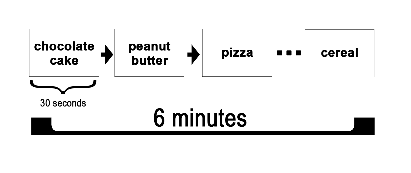
For the MRI ancillary study in this paper, eligible participants completed an in-person screening visit, as well as one 45-minute baseline MRI scan session. During the initial in-person visit, documented informed consent was obtained. Participants also completed an MRI screening form and named their four favorite foods for use in the MRI scanning protocol. For the MRI scanning visit, study participants arrived in the morning after an 8 hour fast. The MRI scan session included a food-cue visualization task. During this task, participants viewed the words of their favorite food items. As each word was presented in 30-second intervals for a total of 6 minutes, participants were instructed to imagine the taste, the smell, and the satisfaction of consuming the food (Figure 1). Resting-state was also performed but are not used in the present study. Participants then went on to receive one of three interventions: (a) mHealth-supported dietary weight loss program with a nutritionist (WL) + structured aerobic exercise (EX); (b) WL + a novel daily movement intervention (SitLess); and (c) WL + EX + SitLess. Of the 71 participants who consented, 9 participants were removed because of excessive head motion, and 4 were removed because of missing 6-month weight-loss data. Therefore, the final sample included 58 participants. The study protocol was approved by the Wake Forest School of Medicine Institutional Review Board. Refer to Table 1 for age, sex, BMI, and weight-loss descriptive statistics. Refer to the supplementary material for plots of the BMI distribution for each group.

Figure 1.Visual representation of the food cue task. Participants viewed the words of their favorite food items. As each word was presented in 30-second intervals for a total of 6 minutes, participants were instructed to imagine the taste, the smell, and the satisfaction of consuming the food.

2.2. MRI Data Acquisition and Processing

MRI data were acquired using a Siemens Skyra 3.0-Tesla scanner with a 32-channel head coil. A single shot 3D MPRAGE GRAPPA2 pulse sequence was used for the acquisition of high-resolution T1 structural images with the following scan parameters: voxel size = 1.1x1.1x1.2 mm, TR/TE = 2300/2.95 ms, FOV =270 x 270 mm, flip angle = 9 degrees, slice number = 176. For the food-cue functional magnetic resonance imaging (fMRI) scan, we used a single-shot gradient echo-planar imaging (EPI) pulse sequence with TR/TE =2000/25 ms, FOV= 256 x 256 mm, flip angle = 75 degrees, slice number/volume = 35 and acquisition length of 434 seconds (217 volumes). The slice thickness was increased from 4 mm to 5 mm during the study as the thinner slices failed to cover the whole brain for several subjects. There was not a statistically significant difference in the number of 4 mm slices versus 5 mm slices between the two weight loss groups (p=\(0.1186\)).

The preprocessing of MRI data was carried out using Statistical Parametric mapping (SPM12) unless otherwise noted. We created atlas-based preprocessed time series in each participant’s native (original) space. First, each subject’s T1 was coregistered to the MNI152 template to improve segmentation and warping. Next, the T1 were segmented into gray matter, white matter, and cerebrospinal fluid.²⁹ The T1 was masked to only include gray matter and white matter tissues (manually correcting any misclassifications in the segments), and the resulting image was warped to the Colin brain template³⁰ using Advanced Normalization Tools (ANTs).³¹ The inverse of the obtained deformation map was used to warp the Shen atlas³² to each subject’s native anatomical image. Finally, the T1 was coregistered with the fMRI scans, and the registration parameters were applied to the inverse warped Shen atlas.

We removed the first 10 volumes from the fMRI data to eliminate the instability of the fMRI signal at the beginning of scans. Next, we performed slice timing correction and scan realignment. A band-pass filter (0.009-0.08 Hz) was used to remove low-frequency scanner drift and high-frequency physiological noise. We then regressed out six motion parameters in addition to the mean brain signal of gray matter, white matter, and CSF using a single regression analysis. Finally, the mean of the processed fMRI signal from each of the 58 Shen atlas regions belonging to FN1 and FN2 was computed and used as input for our hidden semi-Markov model (HSMM) framework (described in Sections 2.3 and 2.4).

2.3. Functional Networks of Interest

For this study, we investigated how individuals traverse in and out of different network topologies at a baseline fMRI scan (prior to weight-loss intervention) involving 58 brain regions from FN1 and FN2 that we had found in prior research to be predictive of future 18-month weight loss in older adults with obesity.¹⁴ In this prior research, these two FNs were identified using machine-learning techniques. However, the machine learning techniques did not identify how shifting in and out of different topologies of these networks was associated with weight-loss; rather, these techniques simply found that networks of these specific regions were associated with weight loss (i.e., what the networks look like and how the networks were traversed by participants was not quantified).

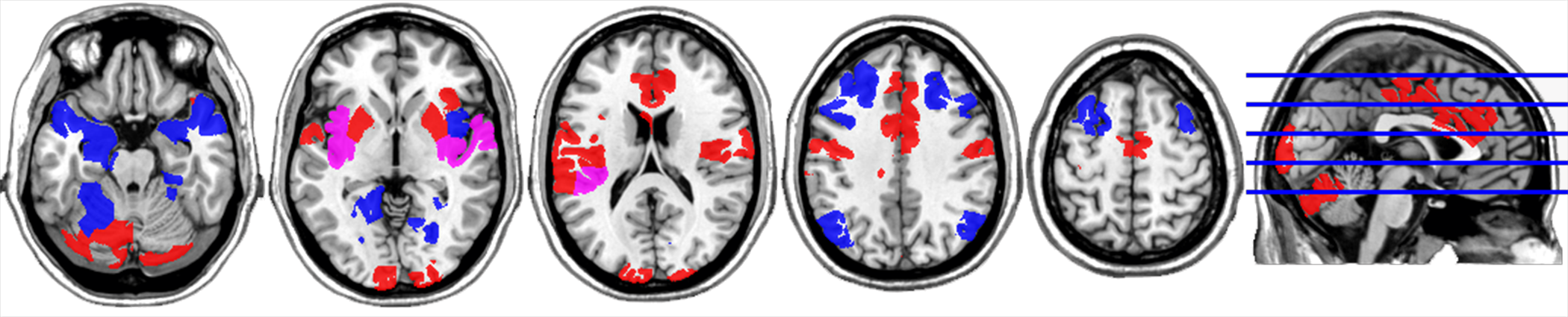
The two FNs contain key regions that play roles in incentive sensitization, reward valuation, and executive function.^2,33 For FN1, the ROIs in the most posterior area of the brain are in the visual cortex, while the nodes in the more anterior locations occupy lateral motor and somatosensory regions, the anterior cingulate, and the posterior insula. The nodes located in the inferior posterior aspect of the brain occupy the cerebellum. For FN2, the ROIs located in the superior aspect of the brain are part of the attention-processing circuit. The nodes in the inferior aspect of the brain localize to the amygdala, temporal pole, hippocampus, fusiform gyrus, and inferior insula. Figure 2 provides a visualization of FN1 and FN2. For a complete list of Shen atlas regions belonging to each FN, please see the supplementary appendix.

Figure 2.Visual representation of the brain regions comprising FN1 (red), FN2 (blue), and regions in both FN1 and FN2 (purple). These are the regions we included in our analyses. Slices shown: 50, 70, 90, 110, and 130.

2.4. Hidden Semi-Markov Modeling (HSMM)

We fit an HSMM on the fMRI ROI time series data of our final sample of study participants. A detailed description of the HSMM can be found in ²⁶, but we provide a summary below.

We denote the ROI time-series data for each participant by \({Y_{i1}}, . . . , Y_{iT}\), where each \(p-\)dimensional vector \(Y_{it}\) contains the BOLD measurements of the \(p\) ROIs at the \(t^{th}\) timepoint for the \(i^{th}\) participant. The collection of vectors of observed time-series data is denoted by \(\tilde{Y_{i}}\). Now suppose a unique, unobservable network state gives rise to each \(Y_{it}\). We represent this unobservable network underlying the observed time-series vectors at a particular observation time by \(S_{it}\). That is, \(S \in {1...K}\), and the vector of true network state variables, \(S_{i1},..., S_{iT}\), is denoted by \(\tilde{S_{i}}\).

We assume that each \(Y_{it}\) follows a multivariate Gaussian distribution \(Y_{it}\sim\mathcal{N}(\mu_{s=k},\,\Sigma_{s=k})\), where the mean and covariance are dependent on the current (unknown) network state \(s\), for any \(S \in {1,...,K}\). Therefore, each network state has its own set of mean activations across our pre-specified ROIs, as well as its own covariance/correlation structure between ROIs. Each state’s correlation structure represents an undirected weighted network.

Not only does the model contain the mean and covariance matrix for each network state, but it also contains parameters that estimate a) transition probabilities between network states and b) sojourn/dwell times for each state. These parameters are important for quantifying the network dynamics and patterns of network state traversal during the fMRI scan. See Supplementary Material for the complete data log-likelihood of the HSMM and Figure 3 for a pictorial representation of the model.

Figure 3.Hidden Semi-Markov Model Overview. The unobserved hidden states evolve according to a semi-Markov process characterized by state transition probabilities (underlying the red arrows) and duration densities/sojourn distributions (dashed lines). The BOLD signals at each timepoint are assumed to follow a Gaussian distribution with parameters that depend on the current network state.

For our main analysis, we fit one set of network states using the data across all individuals in our sample. The number of states one can fit must be specified a-priori and is heavily dependent on the number of participants, number of timepoints, and number of ROIs. As the number of states increases, the number of parameters will similarly increase, as well. Given our sample size, we found that five states produced stable parameter estimates over multiple fittings of the model. Moreover, based on extensive simulations, what we have found is that an inaccurate specification of the number of states can lead to the identification of spurious or merged states.³⁴ Our solution to this problem involves running the model with different numbers of states and examining the Euclidean distance between the states. The distance between the states should indicate how similar or dissimilar the states are. Genuine brain states are very distinct from each other, while the structure of spurious states is very similar to genuine brain states. Therefore, we executed the model with varying numbers of states and subsequently assessed the minimum distance between the identified states in each run. The run exhibiting the highest minimum distance was the 5 state run, indicating that it had the highest distinctiveness in the estimated states (refer to supplement for our plot of the minimum distance for each run).

Additionally, we used a smoothed-nonparametric sojourn distribution for the sojourn/dwell time distribution aspect of the HSMM. This choice is particularly useful for situations where we do not know the exact form of the sojourn distribution, as it does not have a specified analytic form. We initialized the model with a uniform distribution where the parameters were a \(T \times K\) matrix (\(T\) represents the total number of timepoints and \(K\) the number of states). For each state, at each iteration of the maximum likelihood estimation algorithm (described in the next section), a kernel density estimate was computed by first finding which \(t\) in the range \([1, T]\) had a density value that exceeded a smoothing threshold (\(1e^{-20}\)), and then by using the density value at those points together with a Gaussian kernel (for smoothing purposes) to obtain the estimate.

2.5. Maximum Likelihood Estimation

The HSMM parameters were estimated utilizing the mhsmm R package.³⁵ We combined the time-series data of each individual, resulting in a dataset with a total row count equal to the sum of the lengths of all individuals’ time-series data. The dataset had a column count equivalent to the number of Regions of Interest (ROIs), which was 58. Subsequently, the Hidden Semi-Markov Model (HSMM) parameters were estimated using this complete dataset, yielding a single set of model parameter estimates (e.g., the network states). The Expectation-Maximization algorithm was used to estimate all model parameters.

Each participant’s most probable sequence of true network states was estimated using the Viterbi Algorithm.³⁶ The Viterbi algorithm takes as input the state estimates, transition probability estimates, sojourn density estimates, and initial state probability estimates derived from fitting the Hidden Semi-Markov Model (HSMM) on all participants. It then computes the most probable sequence of states for each individual participant based on these estimates and their own BOLD time-series data. Essentially, it discerns, for each time point, the state that the participant’s data suggests they are in among the five states. Hence, while the state estimates are derived from the entire dataset, the dynamic transitions between states are specific to each participant. A further description of the model estimation procedure can be found in H. Shappell et al.²⁶

2.6. Community Structure Analysis

To aid in characterizing each of the 5 network states, we performed a modularity analysis on each state that split the network into distinct, nonoverlapping communities. Modularity indicates the level of segregation in a network by comparing within community connections with respect to in-between community connections. A high level of modularity specifies the network’s ability to be divided into well-defined communities.³⁷ Covariance matrices obtained for each of the five fitted states were converted to correlation matrices, which then represented our undirected, weighted graphs. All negative correlation values were set to 0. The Brain Connectivity Toolbox (www.brain-connectivity-toolbox.net)³⁸ was then used to define the communities. Community definitions were qualitatively compared across states and community labels were matched for comparison purposes.

2.7. Statistical Inference and Permutation Testing

We assessed the relationship between future weight loss (successful vs. unsuccessful) and both occupancy times and empirical sojourn distributions of the brain states inferred from the HSMM using the baseline fMRI data. A participant’s occupancy time for each state was calculated by summing the total number of timepoints spent in that state and dividing by the length of the participant’s time-series, then converting to a percentage. Group averages were then calculated for each state by finding the mean across all participants in each group. From there, an observed group difference (successful minus unsuccessful) was calculated to be used for permutation testing.

To calculate the empirical sojourn distribution of each state for a participant, we counted the number of consecutive time points the participant remained in a given state, each time that they entered the state. We then gathered these counts across all participants in each group and computed a density estimate for each group from the counts. For all calculations involving sojourn times, we left out the starting state sequence and ending state sequence for every individual. We did this to avoid a bias towards shorter sojourn times since we had no way of knowing how long the individual was in the state before beginning the scan or after ending the scan. After obtaining separate empirical sojourn distributions for each group for all 5 states, we performed a group comparison of each state’s empirical sojourn distribution using Kullback-Leibler (KL) divergence, a measure of the directed divergence between two probability distributions. See H. Shappell et al.²⁶ for a more detailed description of the KL divergence in this context. In the simple case, a KL divergence of 0 indicates identical behavior from both distributions, whereas a KL divergence of 1 indicates vastly different behavior. The Philentropy R package was used to calculate the KL divergence.

To determine if any observed occupancy time and/or sojourn distribution differences were statistically significant, we performed a permutation test based on 1000 permuted samples. Permutation testing was chosen over more traditional statistical tests due to its more relaxed assumptions on data distributions, sample size, outliers, and independence.

3. Results

3.1. Functional Brain State Characterization and Occupancy Times

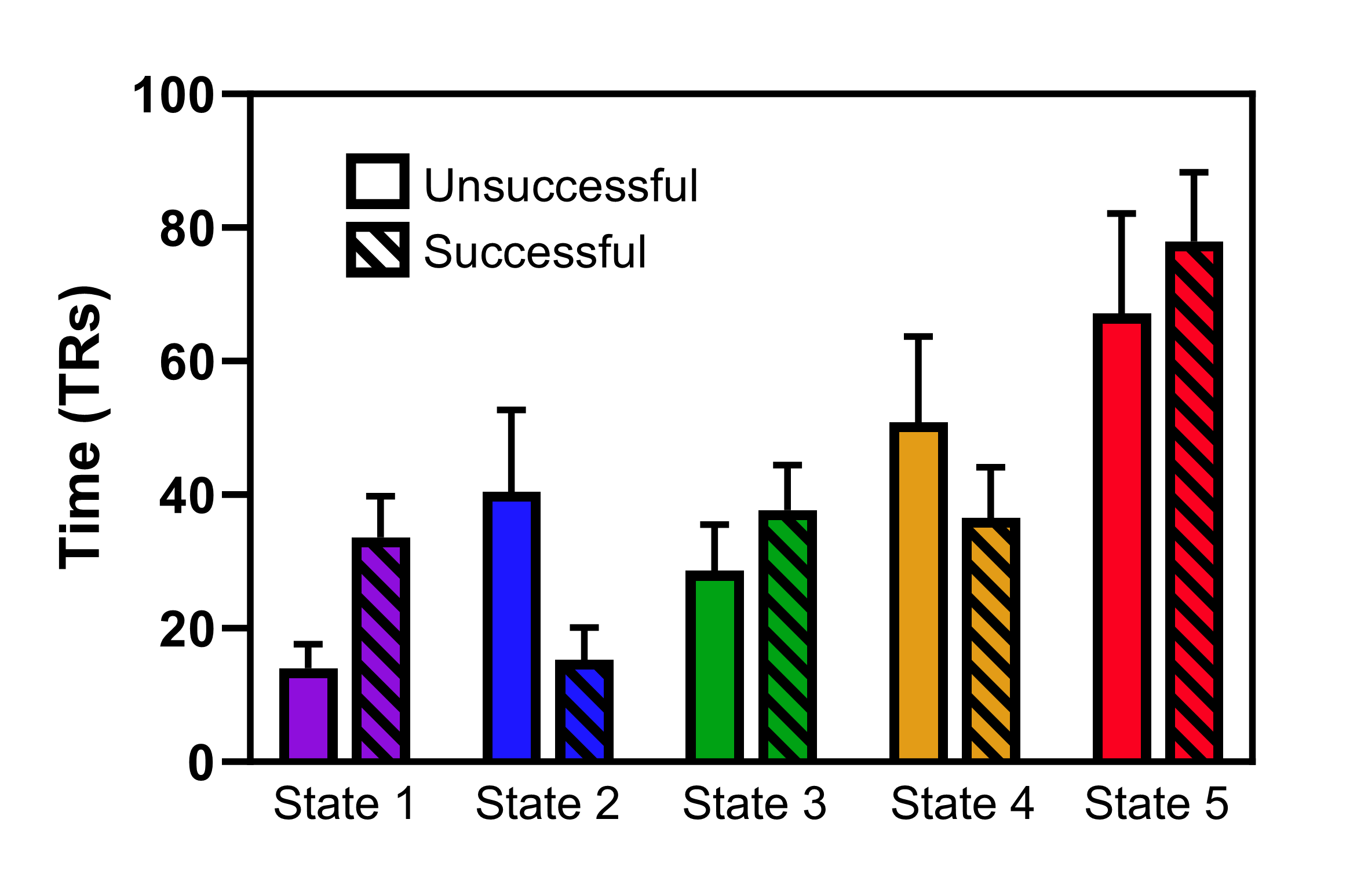
Participants who successfully went on to lose at least 5% of their body weight spent significantly more time, on average, in states 1 and 3 at baseline (\(p-value = .025\) and \(p-value=0.049\), respectively) compared to those who were unsuccessful at losing 5% of their weight (Figure 4). Moreover, participants who did not successfully lose at least 5% of their baseline weight spent significantly more time, on average, in state 2 (\(p-value = .031\)). They also spent more time, on average, in state 4 (\(p-value=0.053\)), but this was only borderline significant. State 5 was the most dominant state, overall, with both groups spending an average of at least 30% of their time in this state, with no significant difference between the groups.

Figure 4.Occupancy times (represented by total number of TRs) for each state for successful and unsuccessful weight-loss participants.

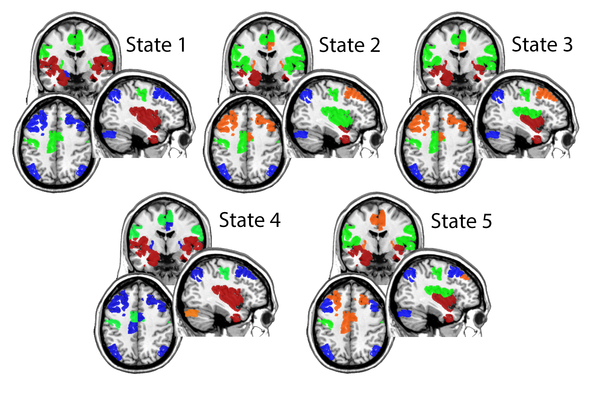
The community membership of each of the 5 states is shown in Figure 5. There were no states that exhibited community structure with FN1 and FN2 each in a single community, as all states had more than 2 communities. State 1 had three communities while states 2-5 each had four communities. The regions encompassed by FN1 and FN2 broke into several meaningful clusters such that there was an overall pattern that emerged across states. This pattern was such that the lateral sensorimotor regions and cingulate regions (likely motor planning) from FN1 (green community) and the limbic regions from FN 2 (red community) were typically each in their own community that may or may not include other state-distinguishing regions. The lateral frontal and parietal regions from FN2 were typically separate from the sensorimotor or limbic areas in a single community (blue community) that also included cerebellum and visual cortex that are part of FN1. When the frontal and parietal were not in the same community, they exhibited an anterior/posterior split forming a unique module primarily containing the frontal regions (but see below). The insula turned out to be one of the most interesting regions distinguishing the different states. It exhibited the most fickle behavior as it changed community allegiance quite dramatically. It was totally aligned with either the sensorimotor or the limbic, or split with more posterior aspects being aligned with the sensorimotor areas and the inferior/anterior aspects being with the limbic areas.

Figure 5.Characterization of Network States. Community structure analysis was performed on each network state, where each color represents a different community in a given state. Community color labels were matched across states for comparison purposes.

State 5 is unique from the other states with the medial frontal regions being split from the remainder of the frontoparietal circuit from FN2. This is the state that both groups spent the most time in on average. In this state, the more medial aspect of the frontal region was in a new community that contained the medial motor planning region as well as the small region of basal ganglia. The lateral frontal remained in the same community as the parietal cortex (a large component of FN2) along with visual and cerebellar regions (FN1). A third community for this state consists of the motor region and the superior insula (the majority coming from FN1). Lastly, a fourth community consists of the anterior inferior insula and limbic regions making up the majority of the inferior aspect of FN2.

States 1 and 3 are the two states that the successful weight-loss group spent more time in, on average, compared to the unsuccessful weight-loss group. In state 1, sensorimotor and basal ganglia regions are in a module together (all FN1 regions). No portions of the insula were in the module with the sensorimotor regions. In contrast, state 3 had the sensorimotor and dorsal posterior insula (mostly FN1 regions) form a module. Lastly, in both states 1 and 3, the insula and limbic structures are well integrated (which consist of the shared FN1 and FN2 regions). In state 1 it is the entire insula with the limbic regions but in state 3 it is the anterior inferior portion of the insula. Figure 6 demonstrates that states 1 and 3 are characterized by strong FN1 connections bilateral between the motor areas (state 1) with additional connections between the motor area and dorsal posterior insula (state 3). These two states are also characterized by positive connectivity between insula and limbic structures. The split of the frontoparietal module in state 3 is noted by the absence of long-range positive connections between frontal and parietal cortex. This is most evident when comparing the sagittal images for states 1 and 3.

States 2 and 4 are the two states that the unsuccessful weight-loss group spent more time in, on average, compared to the successful weight-loss group. State 2 exhibits a striking difference from all other states. In this state, the limbic system (part of FN2) is in a module by itself. This is the only state where this was observed. Additionally, the sensorimotor regions are in a module containing the entire insula (consisting of insular regions found in FN1 and FN2). As shown in Figure 6, the insula nodes have strong positive connections bilaterally and to the sensorimotor regions. Contrast this with state 1, where the insula and motor have some negative connections, rather than strong positive connections. State 4 shares similarities with state 1, having insula and limbic structures in a single module (a mix of both FN1 and FN2), and the frontoparietal module having strong positive connections (i.e., a high level of connectivity within FN2 regions). The major distinctions of state 4 is that the frontoparietal module contains the majority of the cingulate as well as the basal ganglia. In addition, the cerebellum and visual regions from FN1 are in their own module. It is clear from Figure 6 that these posterior areas have many negative connections with the frontoparietal module. In contrast, in state 1 the visual cortex and cerebellum are also highly integrated with the frontoparietal regions.

3.2. State Dwell Times

The sojourn/dwell time represents how long a participant spends in a state before transitioning to another state. Figure 7 presents the sojourn distributions for the five states for each weight-loss group. Higher curves further to the left on the x-axis indicate shorter dwell times for that state. In other words, participants quickly leave the state after entering it. Similar to occupancy times, we conducted permutation testing and found a significant difference in sojourn distributions between the two groups for states 1, 2, and 4 (p-values \(= 0.033, 0.038, 0.046\), respectively). Specifically, we found that successful weight loss participants spent less time in states 2 and 4 before switching out of them. On the contrary, unsuccessful weight loss participants spent less time in state 1 before switching to another state. Group difference p-values for states 3 and 5 were not significant.

3.3. State Transition Probabilities

The two groups of participants differed in how likely they were to transition to each of the other states from their current state (Figure 8). The participants who successfully lost weight cycled between states 1 and 4, whereas those who did not successfully lose weight tended to cycle between states 3 and 5. Successful participants also cycled between 3 and 5, but not as much as the unsuccessful participants. Other notable group differences were that the successful group traversed from state 2 to state 4 more often than the group who was not successful at weight loss. They also traversed from state 3 to state 4 more often than the unsuccessful group. Meanwhile, the successful group transitioned less often from state 3 to state 5 and from state 4 to state 5.

4. Discussion

The intent of this study was to build upon an original investigation of FN1 and FN2 that observed strong longitudinal relationships between these networks and future 18-month weight loss in older adults.¹⁴ Because we identified these networks using time-dependent, dynamic methodology, we reasoned that we could achieve a more in-depth conceptual understanding of how these networks operate by analyzing patterns of changing brain states during the active processing of preferred foods. To this end, we employed novel statistical methods: Hidden Semi-Markov Modeling (HSMM). The results of these analyses yielded 5 different brain states arising during a 6-minute baseline fMRI scan while participants processed individually tailored food cues. There was a dominate state (state 5) that participants occupied an average of 30% of the time regardless of future weight loss success. However, there were 4 other states that distinguished participants who either succeeded or failed to meet or exceed a 6-month, 5% weight loss criterion. We provide the details on these results below.

State Occupancy and Dwell Times

Figures 4-6 captured the 5-state solution resulting from the HSMM and the time during which participants, who either succeeded or failed at weight loss, occupied each state. Figure 7 displayed dwell times: the amount of time spent in a particular state prior to moving to another state. Because there was no statistically significant difference in preference for the occupancy of state 5 on the part of those who either succeeded or failed at weight loss, we propose that it represents a base state of the brain in response to participants’ actively processing sensations associated with preferred foods. In our original machine learning study on data from resting state scans in older adults with obesity following an overnight fast,¹⁴ FN1 and FN2 were largely segregated, independent networks. In this current study, we observe a similar phenomenon in state 5, but with a few strong connections between regions in FN1 and FN2 in the other four states. As shown in Figure 6, state 5 has one of the highest numbers of negative correlations between FN1 and FN2 regions and the lowest number of positive correlations between this same set of regions. It also has the highest positive correlation between ROIs in FN1. The same holds true for FN2. What all of this suggests is that FN1 and FN2 are more segregated with regards to the number of connections between them in State 5 compared to other states. However, the connections that do exist between FN1 and FN2 (e.g., dorsal lateral frontoparietal with visual and cerebellum, as well as the anterior insula and limbic regions with each other) are quite strong. As previously described by Mokhtari and colleagues, FN1 represents a network dominated by interactions between the cerebellum, lateral sensorimotor areas (including face, mouth, and throat), posterior insula, mid-anterior cingulate cortex, as well as the early visual cortex. A diverse group of investigators have found these areas of the brain to be important in the optimization of feeding behavior.^39–42 Alternatively, FN2 captures interacting patterns between the executive attention network and the hedonic/goal directed network including the amygdala, hippocampus, and inferior insula. This network captures regions of the brain central to the process of top-down control that the attention network projects onto the limbic regions known to be important in goal-oriented behavior,^17,18 with connectivity between the control and reward/motivation networks playing a central role in the regulating food consumption.^43,44

Figure 6.Brain Network structures for each of the five states, displaying the edges corresponding to the top three positive and the top three negative correlation values for each node. For each state, glass brain images depict coronal (top), sagittal (middle), and axial (bottom) views. Positive correlations are shown in dark gold and negative correlations are in dark gray. The edge width reflects the correlation values. Vertices are color-coded according to their community assignments from the modularity analysis of the complete positive network. The size of each vertex corresponds to the sum of the positive weights.

Figure 7.Estimated empirical sojourn distributions for each state for the successful and unsuccessful weight loss groups, indicating that successful weight loss participants spent less time in states 2 and 4 (p-values = 0.038, 0.046, respectively) and more time in state 1 (p-value = 0.033) than unsuccessful weight-loss participants before switching to another state.

Figure 8.A visual representation of the conditional transition probabilities between states, as well as the state occupancy times. The top left plot is for unsuccessful weight loss participants, whereas the top right is for successful weight loss participants. The bottom middle figure is the change between groups (unsuccessful minus successful). Edge widths are proportional to the conditional transitional probabilities between states, with thicker edges representing a higher probability. State node sizes are proportional to the occupancy time of each state. We highlighted the five largest conditional probability differences between the two groups with red and blue arrows. Red arrows indicate a higher probability in the unsuccessful group, and blue arrows indicate a low probability in this group.

What stands out in the occupancy data of the other four brain states is that participants who succeeded at weight loss spent more time in states 1 and 3 than those who failed, whereas those who failed at weight loss spent more time in states 2 and 4. It is also interesting to underscore patterns in the dwell time data. Specifically, when participants who succeeded at weight loss moved to states 2 and 4 or those who failed moved to states 1 and 3, they quickly moved out of these states. These patterns in occupancy and dwell times for states 1-4 led us to explore the topographical characteristics of these states.

Characteristics of Brain States 1-4

As noted above, during active imagery of preferred foods, participants who were successful at weight loss spent more time in states 1 and 3. Consistent with state 5, within states 1 and 3, the insula and limbic structures were well integrated, representing shared ROIs between FN1 and FN2, along with ROIs unique to FN2. These novel patterns in dynamic brain states reinforce the crucial aspect of Mokhtari and colleagues¹⁴ work, that is, FN1 and FN2 evolved from machine learning of time dependent, dynamic fluctuations of resting state data, not static networks. The current analyses demonstrated that, as participants actively processed personally relevant food cues during the scanning task, there were important time-dependent brain states that emerged within and between the ROIs captured by FN1 and FN2. Features of states 1 and 3 also included strong FN1 connections, specifically between the motor area, basal ganglia, and cingulate (state 1) and between the motor area and dorsal posterior insula (state 3). As we have recently suggested in a paper that examined connectivity within FN2 during active processing of food cues among these same participants, the executive attention network seems to function as an intermediary between the limbic circuitry and the remainder of the brain, particularly the sensory motor cortex and other ROIs found in FN1. It is well known that the executive attention network is essential to goal directed behavior^17,18; it plays a critical role in regulating food consumption.^43,44 Finally, in cross-sectional analyses, we have shown that FN2 correlates with a measure of self-efficacy related to confidence in resisting the urge to eat.¹⁶

We next turn our attention to states 2 and 4, the higher occupancy states for participants who failed at weight loss. Of particular interest for state 2 was (a) the segregation of the limbic system from other ROIs in FN2, (b) the connectivity between the motor regions in FN1 with the insular cortex, and (c) the frontoparietal breaking into anterior and posterior modules with many negative connections between the modules. Within state 4, the motor regions were in their own module and less integrated with FN2, which contrasted with state 1 where the motor regions had connections to the cingulate and basal ganglia. The frontoparietal areas were more connected with the cingulate and basal ganglia compared to other states. These features of state 2 and 4 are consistent with our prior work suggesting that, in those who struggle with weight loss, the limbic portions of FN2 likely interact with the rest of the brain without using the attention network as an intermediary superhighway. One could argue that, in effective weight loss, the executive attention network regulates how the more primal limbic regions process information rather than allowing the limbic regions to communicate freely with the rest of the brain.⁴⁵

Study Limitations

We found that five states properly fit the data, allowing for variability between the states entered by the successful and unsuccessful weight loss groups. The current HSMM approach works best when estimating the states from the entire combined group so that between group comparisons can be made on the dynamics of these states. In the future, it would be useful to define participant-specific states to allow for as much individuality as possible. In order to do so, however, random effects would need to be incorporated into the HSMM. A mixed-effects HSMM framework will be developed in future work to enable individual state-fitting, as well as to enable covariates such as sex, age, or behavior to be included as fixed effects directly in the HSMM. This would also allow us to directly include our variable of interest (change in body weight from baseline) as a covariate in the model, allowing for a direct statistical test of this variable. While the 5% cut-off we used to define our two groups has clinical relevance,⁴⁶ we are losing information by binarizing our main variable of interest.

As previously described, we focused our analyses on regions belonging to two functional networks (FN1 and FN2) that were shown to be associated with weight loss in an independent data set. While we did this to expand on previous findings involving these regions, it would be ideal to include many more regions that span the entire brain. Unfortunately, the current version of the HSMM approach requires restricting the number of brain regions given our smaller sample size. Inference in HSMMs with even a moderate number of brain regions is a challenging problem because the number of parameters that need to be estimated for each state correlation matrix is \(\frac{p(p-1)}{2}\), where \(p\) is the number of brain regions. This large number of parameters leads to the restriction of the number of brain regions that may be included in the analysis and is partially dependent on study sample size and length of scans. Future work will involve developing an HSMM approach that will allow for much larger network sizes. This model should promote sparsity in the networks, encouraging only the presence of edges between brain regions best supported by the data. This will greatly increase the impact and scalability of the current method, allowing us to study a more complete picture of the brain and enabling a more refined interpretation of results.

Additionally, we should note that while our results provide evidence that brain network dynamics are predictive of future weight-loss success, we cannot make any direct causal claims. Such claims would need to be backed up by a very carefully designed randomized controlled trial.

Lastly, it should be noted as a limitation that the hypotheses and analyses were not pre-registered.

4.1. Conclusions

Whereas early research on the topic of weight loss focused on specific regions in the brain, it has become clear that weight management involves complex connectivity between many regions distributed throughout the brain. ⁴⁷ have shown that two principal functional networks across the brain, labeled FN1 and FN2, capture core conceptual concepts that other researchers have identified as being central to weight management^2,48: reward valuation, incentive sensitization, and executive function. To our knowledge, the current analyses are the first to illustrate the importance of temporal changes in brain networks in the brains of adults with obesity following an overnight fast as they respond to preferred food cues. Of key significance is that participants who went on to either succeed or fail at 6-month weight loss exhibited different occupancy and dwell times for these five states.

From a behavioral perspective these findings underscore the limitations inherent in using static brain networks as predictors of food intake and weight management.¹⁴ Clinically, these data illustrate the challenge of treating participants who frequently come to treatment in sated states, when the real question is how they feel and behave in response to food enriched environments either when they sit down to consume a meal or consume food between meals! The recognition that weight management involves complex temporal shifts in brain states could lead to the development of new treatment options that complement current behavioral methods for weight management which largely rely on conscious, decision-based theories.

Data and Code Availability

Data can be made available upon request with appropriate Institutional Review Board approval and data use agreements.

Code can also be made available upon request without any restrictions.

Funding

This work was supported by the Institute of Biomedical Imaging and Bioengineering (K25-EB032903-01); National Institute on Aging (R01AG051624-03S2); and the Translational Science Center of Wake Forest University.

Conflicts of Interest

All authors report no biomedical financial interests or potential conflicts of interest.