Tractography analysis with the scilpy toolbox

Introduction

We present scilpy, an open-source Python library for diffusion magnetic resonance imaging (dMRI) and tractography processing.

DMRI allows analyzing water diffusion in biological tissues, offering valuable insight into their underlying microstructure. This information can be used to infer complex features, from local, voxel-wise properties to large-scale connectivity patterns, such as the organization of fibers in the brain white matter (WM). The earliest uses of dMRI included basic tractography through diffusion tensor imaging (DTI)¹ and the reconstruction of apparent diffusion coefficient (ADC) and fractional anisotropy (FA) maps.¹ In recent years, the neuroimaging community has developed advanced local reconstruction methods and tractography algorithms,^2,3 along with powerful tools for analyzing the resulting tractograms, which consist of sets of hundreds of thousands or even millions of streamlines. These include, among others, methods for bundle characterization, which involves analyzing the shape of a bundle or its underlying microstructural properties in a chosen population⁴; analysis of tractogram-related metrics (tractometry, profilometry), which focuses on how selected metrics evolve along different sections of a bundle or the whole-bundle⁵; and connectomics, which examines the strength of structural connections between regions of interest (ROIs).⁶ The evolving landscape of analysis methods requires scientific developers to reimplement and provide continuous support to enable new discoveries (see Supplementary Table A1 for definitions of technical terms relevant to this work). In addition to the usual, well documented initial preprocessing steps, including denoising, registration, segmentation, or reconstruction of local anisotropy information, new analysis techniques include performing task-specific tractography, filtering out outlier streamlines, segmenting bundles, preparing connectivity matrices, computing bundle characteristics or underlying dMRI metrics, and more. Here, we present scilpy, a Python library designed to facilitate a wide range of processing steps, with a particular focus on post-tractography analysis. Scripts are well documented and user friendly: most options have suggested default values based on expert knowledge to help even newcomers use the scripts and obtain good results. Scilpy is updated regularly, allowing it to respond effectively to the new methods that are constantly being introduced in the computational neuroimaging domain, and allowing researchers to follow the most recent trends in analysis. It does not aim to replace existing libraries but rather to complement them. It finds its place alongside other well-known libraries and applications in dMRI (DIPY,⁷ MRtrix3,⁸ Tortoise,⁹ DSI Studio,¹⁰ Phybers¹¹) and more broadly in MRI, including FreeSurfer,¹² AFNI,¹³ FSL,¹⁴ ANTs¹⁵ (see Table 1). Scilpy supports many data formats (e.g., nifti, trk, tck), which makes it easy to use in conjunction with other software.

A general overview of scilpy is presented in section 1. The strength and possibilities from its numerous scripts are presented in section 2. In section 3, we showcase pipelines resolving several dMRI tasks of interest through a series of scilpy scripts. Section 4 details the organization and rigorous testing implemented in scilpy. Section 5 illustrates how scilpy can be used in many research collaborations. Finally, the value of scilpy for educational purposes is highlighted in section 6 and future perspectives are discussed in section 7.

Section 1: The scilpy library

Scilpy has evolved from a private in-house repository into a renowned, robust, and publicly available library. It was created in 2012 as an internal collection of scripts of the Sherbrooke Connectivity Imaging Lab (SCIL). It was initially hosted on Bitbucket, then transferred to a public GitHub repository (https://github.com/scilus/scilpy) in February 2018, and the Bitbucket version was archived. It is supported by a team of over 30 contributors and developers, many of whom are students and collaborators of the SCIL, in Sherbrooke, Canada. Scilpy works on both Linux and macOS and can be installed through PyPI. Scilpy is coded in Python, an easy-to-read, open-source programming language. Some functions requiring faster processing are coded in Cython.

Scilpy aims to be easy to use, and thus both the scripts and the Python functions are well documented, and all descriptions can be found online through the automatically generated API documentation (https://scilpy.readthedocs.io). The website also provides a list of tutorials and examples of typical sequences in the use of the scripts. Scripts are prepared to offer a single task per script, making it easy to separate the scripts into categories (see Table 1), giving a clear overview of the possibilities. Scilpy provides a detailed explanation of required and optional arguments in all scripts. Default, well-tested values that work for a large set of healthy human adult brain analyses are provided. These values have been modified to analyse other populations, such as pediatric¹⁶ or Alzheimer’s¹⁷ cohorts, but the scripts provide only limited support for animal brains. Users can access any script’s documentation via its “–help” option in the command line. Additionally, the script scil_search_keywords helps look for keywords throughout all scripts. As for the Python functions, their docstrings include a summary, expected input parameters, and a list of outputs.

Section 2: Relevance of scilpy for the computational neuroimaging community

Scilpy offers to the neuroimaging community a library with tools covering nearly all preprocessing or postprocessing steps in dMRI, from local modelling to bundle analysis. Users may wonder when to choose scilpy over other libraries. Scilpy does not aim to replace other available tools, but rather to complement them. A general overview of our scripts and how they compare with other libraries in the dMRI field is presented in Table 1.

The first necessary distinction is between scilpy and DIPY.⁷ Scilpy serves as a platform for rapid development, offering access to new tools and enhancements that may not yet be integrated into DIPY.

Throughout the years, many tools were developed in scilpy before being mature enough to be moved into DIPY (e.g., the full spherical harmonics [SH] basis, the asymmetric peak direction, the Bingham model, the Stateful Tractogram, the option to save seeds in .trk files, and so on). To compare the current state of both libraries, we can discuss scripts and Python functions. Regarding scripts, DIPY offers workflows accessible in command-line interface (CLI), similar to our scripts. In particular, they offer options for local reconstruction methods and the tractography algorithm. In those cases, our scripts allow access to the same core functions, sometimes with added detailed documentation. But we also have other scripts that we created to answer needs in the community (see section 5), and we offer many post-tractography analysis scripts. Some scripts are 100% original, others rely more heavily on DIPY, but even in those cases, we complement DIPY by offering management of default values, management of data loading and saving, verifications of input requirements (e.g., header compatibility across files), and often management of computer resources to allow multi-processing. In Supplementary Table A2, we list the DIPY functions accessed in our scripts. Regarding functions, both scilpy and DIPY are mainly Python libraries, and we ensure that our libraries are compatible. For instance, scilpy uses DIPY’s data object structures (e.g., Stateful Tractograms).

The second important comparison is between scilpy and other libraries. In Table 1, we describe the strengths and limitations of scilpy for each category of scripts. In general, scilpy particularly excels in tractogram and bundle operations. We only offer a few options for dMRI volume denoising, segmentation and registration, but other libraries already offer many strong tools (e.g., FSL,¹⁴ ANTs¹⁵ and others). Similarly, we offer a few visualization scripts but no real complex interactive visualization tools. Other libraries already offer good options (e.g., MI-Brain, MRtrix’s mrview⁸ or FSL’s fslview¹⁴). MRtrix⁸ should be mentioned in particular as a similar library to scilpy. It also offers local reconstruction, tractography, and connectomics analysis, but it currently does not support tractometry or profilometry analyses. It does, however, provide options for fixel analysis. We cannot provide a thorough efficiency comparison (computer resource requirements, processing time, quality of the results) because this would require testing all options of all scripts, and comparing results against a ground truth, which is a known limitation in our field.²² But it is worth mentioning that their tractography script runs faster. This is a consequence of the choice of language (MRtrix uses C++), but we believe that using Python helps in making dMRI accessible to newcomers for educational purposes (see section 6).

We note that scilpy supports many data formats to allow compatibility with other libraries and offers scripts to convert volumes or tractogram files.

Scilpy fills a need in the community. Examples of the usefulness of scilpy already appear in the literature. Bundle filtering tools have been used to segment and score bundles in comparison to a reference²³ and to analyse WM in aging²⁴; tractometry (and profilometry) tools have allowed investigations of tau pathology²⁵; and connectomics tools have been used to analyse connectivity alterations in epilepsy.²⁶

Section 3: Including scilpy into scientific projects

An important aspect of scilpy is its emphasis on ensuring that each script performs a single, well-defined task. This granularity leads to a very high number of scripts but allows users to manipulate data exactly as they want. To organize processing steps in their favorite order or to automate processes, for a single subject or for larger databases, users may use their favorite technology. Options range from simply aligning command lines sequentially in a bash script to using more complex workflow management systems such as Nextflow,²⁷ Nipype,²⁸ snakemake,²⁹ and more, which allow parallel processing over various subjects for accelerated workflows. nf-neuro (https://github.com/nf-neuro) is our team’s take on a Nextflow-based pipeline and will be the subject of an upcoming publication. Users interested in processing large cohorts may also discover Tractoflow,³⁰ which includes 26 scilpy scripts and has already led to the creation of multiple-subject databases of processed data.^31,32

We note that the efficiency of pipelines often depends on a clear database organization. Again, this is out of the scope of scilpy, and interested users may find instructions for best practices in other references, such as BIDS.³³

In sections below, we showcase a few examples of analysis objectives and the sequence of scripts required to achieve them. The bash scripts associated with each task are available in the online tutorials.

Objective 1: From raw data to DTI, fODF, and full tractogram

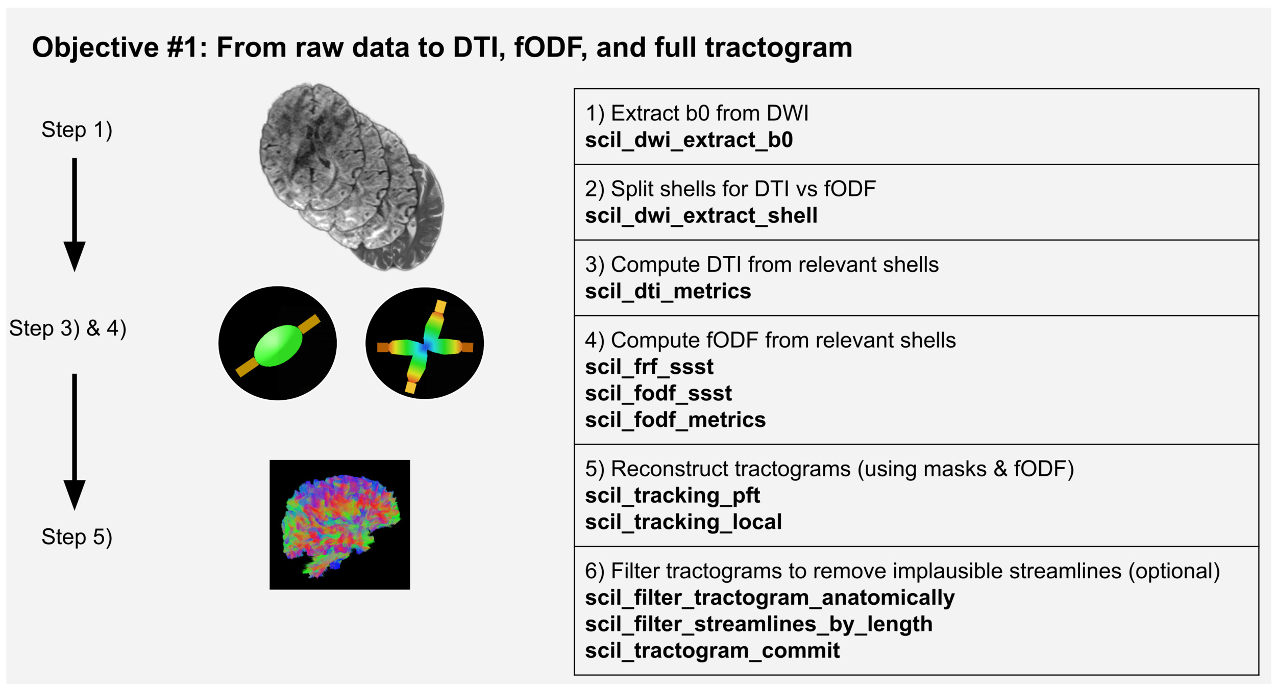
Scilpy scripts allow the complete processing of raw dMRI data in NIfTI format to obtain a full tractogram, such as shown on Figure 1. A complete tractography process can be separated into subsections including 1) a general organization of data, 2) preprocessing and denoising of the DWI data, 3) computation of the local representation, 4) tractography, and 5) filtering out improbable streamlines.

1) During data organization, the user prepares the b-values and b-tensors text files, extracts the b0 and/or the reversed-b0 from the DWI using scil_dwi_extract_b0, and may choose to modify the DWI file in order to improve and facilitate the next processing steps with scripts such as scil_volume_crop, scil_volume_resample, or scil_dwi_concatenate.

2) Preprocessing of the DWI can include rejecting problematic volumes with scil_dwi_detect_volume_outliers or denoising with scil_denoising_nlmeans. The user may include other preprocessing steps of their choice, such as registration to the MNI template with ANTS or skull-stripping with FSL. The computation of the local representation requires the user to first convert the raw signal to SH using scil_dwi_to_sh.

Figure 1.Sequence of scripts to generate a full tractogram from raw data (Objective #1).

Simplified example of a pipeline used to generate a full tractogram from raw DWI data in NIfTI format. This pipeline can be expanded with more advanced preprocessing and reconstruction options. For instance, volumes can be cropped or resampled, and DWI data can be concatenated or checked for outliers before reconstruction. Beyond the DTI and single-shell fODF models shown, scilpy supports various local reconstruction methods, including diffusion kurtosis imaging (DKI), multi-shell and multi-tissue fODF models, NODDI, and q-ball ODFs, allowing for a more detailed characterization of the tissue microstructure.

3) Scilpy has scripts to compute various local reconstruction methods (scil_dti_metrics, scil_dki_metrics, scil_​qball_​metrics, scil_​freewater​_maps, scil_​NODDI_​maps),^1,34–37 particularly many variations of fODFs (scil_​fodf_​metrics, scil_​fodf_​msmt, scil_​fodf_​memsmt, scil_​fodf_​ssst).³⁸ Figure 1 shows an example using fODFs as the local representation, while also computing DTI to obtain crucial information such as the FA map. At this stage, the user may use these results for further analysis such as fixel analysis (scil_bingham_metrics).³⁹

4) The next step is the tractography. Our main tractography script, scil_tracking_local, gives access to all of DIPY’s efficient Cython-based tracking options, and more, such as particle filtering (PFT), parallel transport (PTT) and Euler deterministic (EuDx). Alternatively, scil_tracking_local_dev uses a slower Python loop, but is closer to how one would teach tractography to a newcomer, and allows easy testing of improvement ideas for new developers. Furthermore, this script offers an accelerated GPU-based option or multiprocessing on CPU. Finally, the user could choose to compare results with any other library’s tractography. In particular, scilpy allows saving the fODFs in a SH basis, compatible with MRtrix3 to use their tractography, and conversely, it can perform tractography on fODFs from MRtrix3.

5) The resulting tractogram usually requires postprocessing steps, such as the manipulations described in Objectives #2 - #4. The user could also choose to continue their pipeline with other libraries: our tractography scripts enable saving tractograms as either TRK or TCK to facilitate interoperability with any software accepting these standard formats.

Objective #2: Tractogram manipulations

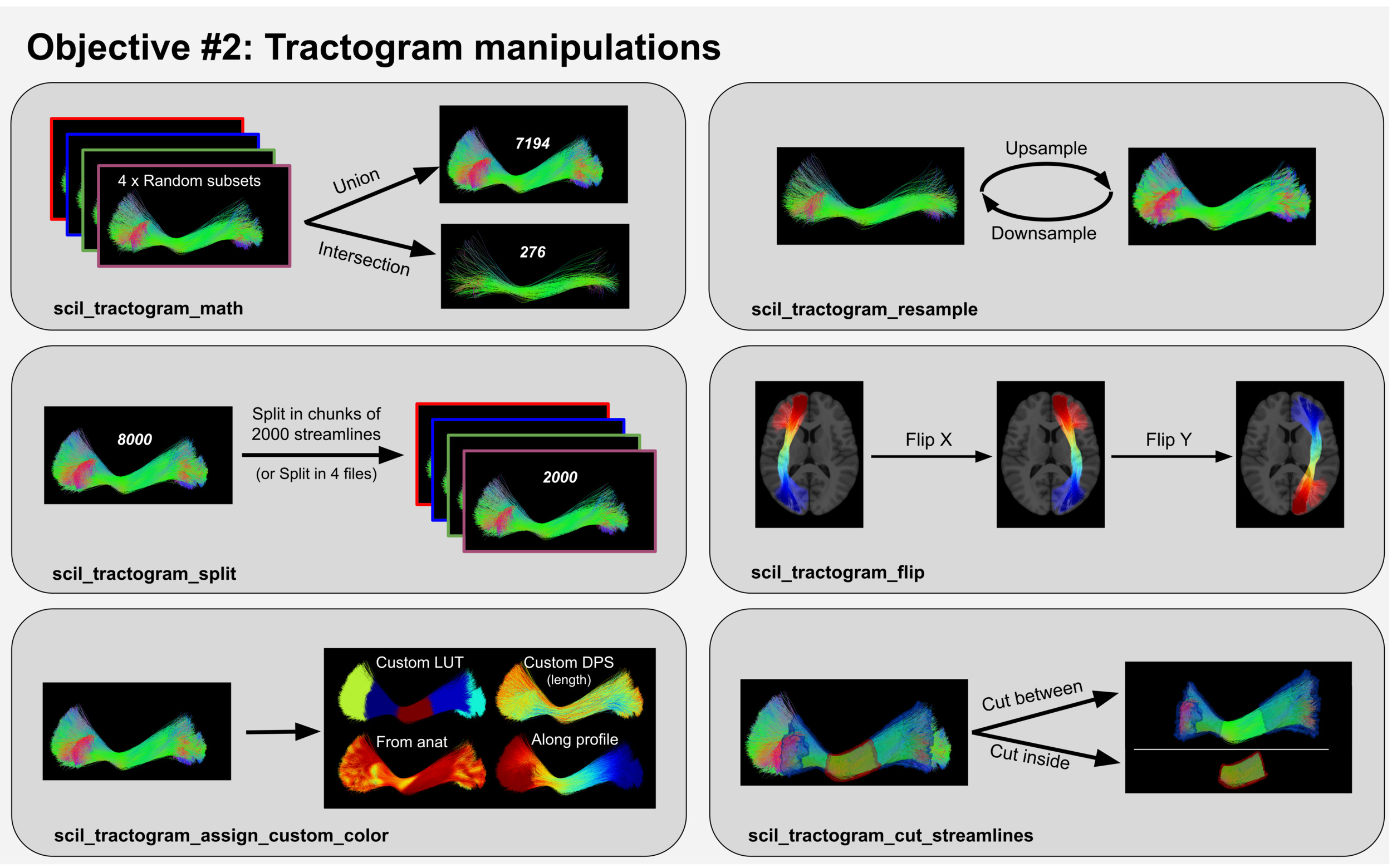
Scilpy scripts allow users to modify tractograms in various ways based on their needs, such as shown on Figure 2.

Some scripts allow operations on the tractogram as a whole object in the brain, such as flipping it on a chosen axis (scil_tractogram_flip) or creating a map of all voxels touched by a streamline (scil_tractogram_compute_density_map). Mathematical operations on two tractograms such as union, intersection, and difference can be performed through the scil_tractogram_math script.

Other scripts allow operations on the tractogram as a set of streamlines, such as resampling the number of streamlines (scil_tractogram_resample, scil_tractogram_split), separating streamlines based on various criteria (scil_tractogram_filter_by_roi, scil_tractogram_filter_by_anatomy, scil_tractogram_filter_by_length, scil_tractogram_filter_by_orientation) or segmenting a tractogram into bundles (see Objective #3).

Finally, other scripts allow modifying the streamlines themselves, for instance by resampling the number of points on each streamline (scil_tractogram_resample_nb_points, scil_tractogram_compress), or smoothing the streamlines’ trajectories (scil_tractogram_smooth).

Furthermore, when using the .trk format, additional information may be stored in memory for each streamline (data_per_streamline [dps]) or for each individual point (data_per_point [dpp]). It is possible, for instance, to store the seeding point of each streamline as dps during the tractography and use it later to create a map of all seeding points leading successfully to a streamline (scil_tractogram_seed_density_map). It is also possible to store a RGB color to each point as dpp, associated to the keyword ‘color’, which allows to visualise the tractogram as desired on a visualization software (e.g., Mi-Brain⁴⁰ supports the ‘color’ keyword). Finally, is it possible to perform more complex actions when analysing some metrics of interest along the streamlines, as described in Objective #4.

Figure 2.Examples of tractogram manipulations (Objective #2).

Scilpy scripts allow modifying tractograms (bundles or whole brain) in various ways. Since our scripts do simple operations, they can easily be chained together to achieve complex tasks.

Objective #3: Creating a WM bundle population template and visualizing it

Scilpy scripts enable users to create a WM bundle population template (see Figure 3). Such a pipeline includes 1) segmenting the bundle of interest in each subject’s tractogram, 2) registering the bundles to a reference space (e.g., MNI space) and analysing the inter-subject variability, 3) combining them into a reference bundle template, similar to how one would average many structural MRI images to create a brain template, and 4) analysing the results.

1) The segmentation of bundles can be based on ROIs of inclusion or exclusion (scil_​tractogram_​segment_​with_​ROI_​and_​score or scil_​tractogram_​filter_​by_​roi) or based on the general shape of the streamlines (scil_​tractogram_​segment_​with_​recobundles, scil_​tractogram_​segment_​with_​bundleseg).^41,42 The resulting bundles can be cleaned more thoroughly than whole-brain tractograms, considering that their shapes should be quite uniform, and spurious streamlines can be discarded automatically with scil_​bundle_​reject_​outliers or visually with scil_​bundle_​clean_​qbx_​clusters. The bundle could also be cut or trimmed using a binary mask, allowing it to focus on a specific region, using scil_​tractogram_​cut_​streamlines. Optionally, metrics and statistics can be measured for each individual subject using our various scripts for bundle analysis, such as presented in Objective #4.

2) Then, registration can be performed by computing the registration matrix between the subjects’ space and the reference space (e.g., using ANTS) and applying the same registration matrix to the tractogram’s coordinates with scil_tractogram_apply_transform. Inter-subject variability can be measured with scil_tractogram_pairwise_comparison.

3) The tractograms can be downsampled and concatenated, as described in Objective #2, and even concatenated to their flipped version to obtain a symmetrical template.

Figure 3.Sequence of scripts for the creation and visualization of a template bundle (Objective #3).

Scilpy scripts allow creating a reference bundle template for a given population. The example above uses a ROI-based segmentation, but other options are available. Once the bundles are clean and registered to a common space, they are downsampled to save space before concatenating all subjects together and performing statistical analyses. It is possible to visualise the inter-subject variability by loading individual tractograms in a visualization software, or to view the spatial range of the population template and its density in each voxel.

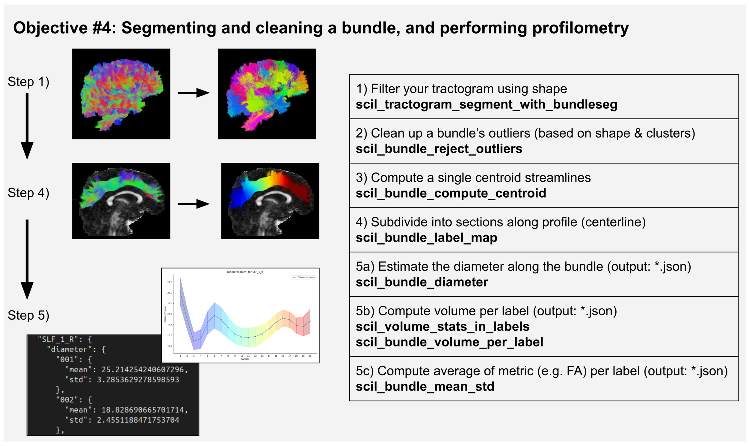
Objective #4: Segmenting and cleaning a bundle, and performing profilometry

Using a clean bundle from a single subject, scilpy allows performing a profilometry⁵ analysis, which is the analysis of the evolution of any dMRI metric along its subsections. A simple example is shown in Figure 4, and for further examples of such processes, users can refer to Tractometry-flow (https://github.com/scilus/tractometry_flow), a Nextflow process using many scilpy scripts, or to the study by Cousineau et. al.⁴³ Such a pipeline includes the same subsections as in Objective #3 (segmentation and cleaning of the bundles of interest in each subject), and analysis of the resulting bundles.

The profilometry analysis requires segmenting the bundles into as many subsections as desired. This is not straightforward, as the division of sections can be performed arbitrarily. We generally cut the section perpendicularly to the direction of the bundle, measured from a centroid, a single streamline-like shape representing the average of all streamlines in the bundle (scil_bundle_compute_centroid, scil_bundle_label_map). Then, any metric can be associated with the subsections. Figure 4 shows the example of the sections’ volume and diameter, or mean underlying value of any given map, such as the FA map. The resulting .json file’s values can be plotted with scil_plot_stats_per_point.

Beyond profilometry, other analysis steps could also be performed on the whole bundle. For instance, it is possible to compute the map of the head and tail of a bundle (the starting and ending regions of the bundle, assuming all streamlines are aligned in the same direction) with scil_bundle_uniformize_endpoints and scil_bundle_compute_endpoints_map. It is also possible to extract various information with scil_bundle_shape_measures.

Figure 4.Sequence of scripts allowing to perform profilometry (Objective #4).

This sequence of scripts allows performing profilometry for a bundle extracted with BundleSeg.⁴⁴ Here, a single cleaning step is performed (step 2), using a hierarchical clustering method.⁴⁵ In steps 3 and 4, the bundle is subdivided into sections (using a centroid to determine a Euclidean association). Finally, step 5 allows quantifying each section of the bundle (shape, volume, metrics, etc.). The JSON output allows easy plotting using any library or conversion to Excel spreadsheets.

Objective #5: Analysing connectivity

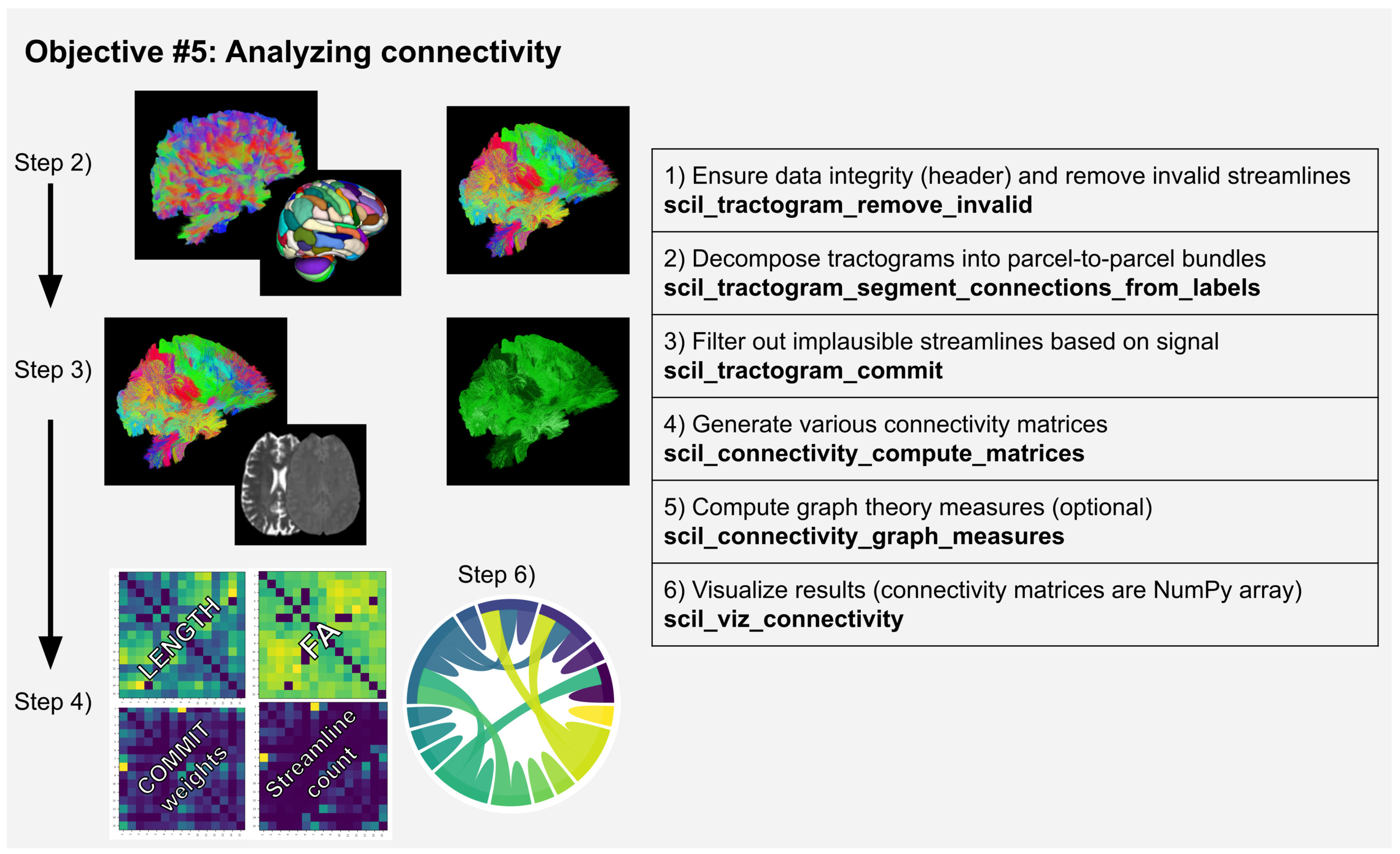
Connectivity analyses use whole-brain tractograms segmented based on a gray matter (GM) parcellation to create various connectivity matrices (see Figure 5).

For a very simple computation, the GM label associated to each endpoint of the streamlines can be used to create a connectivity matrix based on streamline count with scil_connectivity_compute_simple_matrix. However, scilpy also offers a more thorough analysis, with a more complex analysis of endpoints and more options for the weight of the connectivity matrix. It comprises the steps described below.

Figure 5.Connectivity analysis (Objective #5).

Connectivity analysis uses parcel-to-parcel bundles, computed at step 2. After step 4, various connectivity matrices are computed. Steps 5 and 6 are useful to obtain statistics from the matrix.

First, the script scil_tractogram_segment_connections_from_labels is used and results in many sub-bundles, one for each pair of GM regions (each pair of labels). This is similar to ROI-based segmentation, but its computation makes a more complex analysis in cases where streamlines cross many GM regions. The output is saved in the HDF5 format for the ease of use in subsequent scripts but can be converted back to a list of .trk files with scil_tractogram_convert_hdf5_to_trk. Any manipulation can be performed on the bundles and then they could be merged back (scil_tractogram_convert_trk_to_hdf5). Note that bundle registration and analysis presented before could also be computed directly from the resulting HDF5 format, such as warping (scil_tractogram_apply_transform_to_hdf5) or statistics computation (scil_bundle_mean_fixel_afd_from_hdf5).

Then, it is possible to compute the connectivity matrix, using scil_connectivity_compute_matrices, using many weights such as the streamline count, the lengths of streamlines, the volume of bundles, or the average of any underlying map or any dps/dpp stored in the data.

It is possible to modify the matrices afterward with scripts such as scil_connectivity_math (operations such as threshold, addition, multiplication, interchanging rows, etc.), scil_connectivity_filter (to binarize a list of matrices based on conditions) or scil_connectivity_normalize (to modify the minimum and maximum values).

Section 4: Organization of functions, testing, and maintenance

By using Python as the coding language, scilpy benefits from integration with widely used and well-tested opensource packages such as NumPy⁴⁶ (array operations), SciPy⁴⁷ (scientific computing), NiBabel⁴⁸ (neuroimaging file management), and DIPY⁷ (denoising, white matter local reconstructions, tractography algorithms, bundle analysis and spatial transform management of tractograms).

In scilpy, the functions are organized into clearly defined modules (Python files), making it easy to understand the library’s structure. Separation of functions into modules generally follows the separation of scripts into categories (see Table 1). Scilpy’s modular structure allows users to reuse and integrate the functions in scilpy in their projects effortlessly.

Scilpy has rigorous testing code through unit tests and smoke tests in order to ensure its robustness and reproducibility. Smoke tests are minimal tests ensuring that all options in scripts are properly handled and that all scripts can run from start to finish without error. As of October 2025 (version 2.2.1), code coverage covered by smoke tests is 70%. Our goal is to reach approximately 75% coverage for smoke tests. Unit tests ensure that the results of individual functions are as expected, based on numerical results. If analytical testing is not possible, scilpy’s unit tests confirm that the resulting output values remain consistent across versions. Current coverage by unit tests is at 29% for the library codebase. These tests were added recently to the project, in response to scilpy’s increasing recognition and usage, and unit test development is ongoing. Our goal is to reach 100% of our main functions, meaning functions that use DIPY sparsely (DIPY already tests its functions thoroughly) and functions that are not used for visualization, which is difficult to test actively. Modules lacking smoke tests are visualization (cannot be tested automatically) and machine learning (recently added to scilpy). Modules lacking unit tests are post-tractography modules, but, again, development is ongoing.

Section 5: Ease of collaboration using scilpy

Scilpy’s development team has a vision that supports the rapid implementation of new ideas. Scripts are primarily designed to meet user needs.

For example, a common development scenario starts with a collaborator with limited or no computer programming background requiring a specific feature. For instance, they might request a coloring tool where each streamline is colored according to its minimum distance to any streamline within a template, using a designated colormap. This request prompts a discussion regarding input and output data, the required reference frame for the operation, and performance considerations (speed, robustness, and ease of use). The design principles include having the minimal set of arguments necessary towards both collaborator satisfaction and script reusability. The development process begins with a proof-of-concept implementation, which is then shared with the collaborator for iterative refinement, bug reporting, and improvements to the documentation. A context-agnostic development team member reviews the new script to simulate the experience of a new user, emphasizing usability and operational behaviour. Subsequent reviews address code optimization, modularity, input/output handling, general code quality, and implementing unit tests and smoke tests. This entire process typically takes a few weeks. Pull requests are generally merged in a timely fashion and usability can be further enhanced over time as the script is reused and refined based on feedback from subsequent collaborator requests.

The objective of scilpy is to have regular releases. This does require a soft reviewing style but ensures the quick inclusion of collaborative work to our system. On the contrary, DIPY works with a stronger reviewing process and more rigorous code style, resulting in a slower release frequency. Such stricter requirements are necessary due to DIPY’s more widespread use and its functions being used as a foundation for hundreds of projects in multiple labs across the world, and the need to ensure stability for the users. In contrast, the faster release frequency in scilpy helps developers adapt better to rapidly evolving scientific and clinical research projects. Scripts that are not yet fully tested have disclaimers in their description.

Section 6: Scilpy for educational purposes

Scilpy has been designed with a strong educational component in mind. Firstly, it allows research students and collaborators to quickly become familiar with the implementation of complex theoretical aspects in dMRI and MRI data management concepts (3D/4D volumes, tractograms, etc.) by providing a rich set of code examples with integrated input/output from common toolboxes. The use of Python as a programming language also facilitates contributions due to its ease-of-use. Cutting-edge features can mature and survive their contributors by being integrated early into scilpy. Secondly, scilpy’s audience (graduate research students, scientific and clinical researchers, computational scientists, and self-paced curious individuals) can leverage years of expertise in dMRI, embedded into the default parameters, to quickly develop a prototype of their ideal/needed processing pipeline, regardless of their proficiency level. Finally, scilpy is a core component of the SCIL, acting as both a practical tool and a reference implementation for members and collaborators. It embodies and promotes good coding practices and open-source principles, helping to advance the field of dMRI and tractography while raising the standards of the scientific contributions it supports in terms of robustness, reproducibility, replicability, and generalizability. These three educational components help increase scilpy’s educational, scientific, and academic impact.

Section 7: Limitations and future perspectives

We expect scilpy to continue evolving based on collaborations and research projects at the SCIL. Having high-quality documentation and examples are key to its adoption and success, and we intend to build a set of tutorials in the near future. Training the next generation of researchers is important, and we intend to offer workshops on dMRI data processing using scilpy tools and others. We aim to attract new developers to contribute to scilpy through its public GitHub repository.

Although many scripts already offer multiprocessing options, current limits in scilpy’s scripts include RAM management and optimization. We continue actively improving our scripts with every new collaboration. Another limitation from our choice of organization, is that having single-step scripts inevitably creates many intermediate files that would not necessarily be stored on disk with more pipeline-like scripts doing multiple steps at once. This effect can be mitigated with good processing practices.

Conclusion

Scilpy offers unique scientific contributions, addresses critical needs in the computational neuroimaging field, and exemplifies the diverse impacts that open science can have on academic research. Scilpy will help the dMRI scientific community achieve its goals by accelerating the data processing, with a wide range of well documented scripts that cover many scientific and clinical researchers’ needs, and with an easy development process through open-source Python programming.

Data and Code Availability

All code is available publicly on GitHub or PyPI.

Acknowledgements

Thanks to Yuzhe Wang, Hermela Gebremariam, Élise Cosenza, Florence Gagnon and Alexandre Gauvin for their contribution in the Github repository. We would like to thank Kurt Schilling for his useful comments on the text.

Funding Sources

Authors MD and FR thank their respective NSERC Discovery grants (RGPIN-202004818) and the Université de Sherbrooke institutional research chair in neuroinformatics.

Conflicts of Interest

MD is co-founder and shareholder at Imeka Solutions. He has no conflict of interest with respect to the content of this manuscript. All other authors have no conflicts of interests to declare.