Assessing optimisation of 3T MRI protocol across multi-site, multi-vendor settings for studying mild Traumatic Brain Injury: mTBI Predict Consortium study

Introduction

Large-scale, multisite, multivendor, and multimodal longitudinal imaging studies are crucial in brain research for identifying imaging biomarkers across a wide range of brain health issues, including neurodegenerative disorders, mental health conditions, and brain injuries.^1,2 Among these, various brain health challenges stand out as significant global health and societal concerns. Over the past few decades, large-scale imaging initiatives have played a pivotal role in fostering international collaboration in addressing important brain health challenges. Multisite studies enable the inclusion of larger, more diverse sample sizes, enhancing the reliability and generalisability of findings. By integrating multisite data, these studies provide a robust framework for identifying and validating potential imaging biomarkers with greater rigor and statistical power.^2,3

Despite the extensive global burden of mortality and morbidity associated with traumatic brain injury (TBI), most previous TBI studies face challenges due to relatively small sample sizes, which hinder scientific advancement and clinical translation because of the heterogeneity of symptoms and representativeness of included patients.⁴ Neuroimaging studies play a vital role in quantifying pathological changes in TBI that can progressively occur over a prolonged period. Mild TBI (mTBI) is the most common type of TBI, but many cases go undiagnosed because symptoms can be subtle and may not appear immediately. Indeed, no obvious changes on standard clinical MRI scans are one of the diagnostic criteria for mTBI.⁵ This underdiagnosis can lead to untreated symptoms, prolonged suffering, and delayed return to previous work or leisure activities.⁶ If undiagnosed or not fully recovered before patients return to work or leisure activities, they may be at greater risk if experiencing a second concussion, also known as Second Impact Syndrome, which can result in fatal outcomes.⁷ Additionally, if a concussion is not properly managed, the risk of developing psychiatric disorders increases over time due to ongoing disruption in brain regions responsible for mood, affect, and executive function.⁸ Among all neuroimaging tools, quantitative analysis of magnetic resonance imaging (MRI) data, moving beyond visual inspection of structural MRI images which are typically performed clinically, has significant potential to improve clinical assessments and guide the management and treatment of patients following mTBI.^9–11 Therefore, large-scale MRI studies are essential, for providing robust, quantitative data needed to improve our understanding of mTBI, facilitate the development of more accurate diagnostic and prognosticating tools, and ultimately enhance clinical outcomes.

Currently, several global consortia are addressing various issues related to TBI. These include: (i) Transforming Research and Clinical Knowledge in Traumatic Brain Injury (TRACK-TBI)¹⁰; (ii) and Enhancing NeuroImaging Genetics through Meta Analysis consortium¹²; (iii) The Collaborative European NeuroTrauma Effectiveness Research in Traumatic Brain Injury¹³; (iv) Concussion Assessment, Research and Education consortium¹⁴; (v) International initiative for TBI Research¹⁵; and (vi) the Chronic Effects of Neurotrauma Consortium.¹⁶ These consortia address different aspects of TBI research by integrating clinical, genetic and neuroimaging data to improve classification and outcome prediction. While all of them are collecting MRI data, there is notably, limited published research on the initial development of their MRI sequences, and most available studies focus on their applications after protocol standardisation. The TRACK-TBI study protocol for 3T MRI, implemented across General Electric, Philips, and Siemens scanners,¹⁰ was adapted from the Alzheimer’s Disease Neuroimaging Initiative (ADNI)¹⁷; however, it did not include a dedicated optimisation framework. Similarly, the Chronic Effects of Neurotrauma Consortium was intentionally aligned with both ADNI and TRACK-TBI-2, employing relatively comparable 3T MRI acquisition parameters, though detailed protocol information was not provided.¹⁸ The Concussion Assessment, Research and Education consortium’s MRI protocol, developed for Siemens Trio and General Electric scanners, conducted a stability analysis involving 30 and 35 non-contact sport control subjects, and included first two travelling human heads to evaluate site-to-site variation.¹⁹

Multisite and multivendor data acquisition in neuroimaging studies can present significant challenges, including increased variability among scan sessions, differences in MRI sequences across scanners and vendors, and motion biases inherent to different scanners.² These factors can impact the reliability and consistency of the scans, potentially leading to data that is less comparable across sites, which is detrimental to the identification of biomarkers.²⁰ To address these challenges, it is crucial to optimize MRI sequences to minimise between-site differences. This is often done using a “travelling head” paradigm where the same participant(s) are imaged on the different MRI scanners to be used in the main study.²¹ This approach is necessary because MRI sequences often differ inherently between scanner vendors.^1,22 By employing “travelling head” participants, researchers can assess the impact of scanner differences on key metrics that inform future biomarkers. This enhances the reliability and consistency of the data collected across different sites by reducing the impact of scanner-specific biases.^22,23

The mTBI-Predict consortium, of which this work is part, aims to identify the most accurate, and reproducible biomarkers to better identify, in the acute stage (3 weeks) post-mTBI, those at risk of chronic health issues 6 months after the injury. The scale of the mTBI-Predict Consortium’s aims, which includes the recruitment of 610 patients, necessitates a multisite approach, similar to other TBI consortia acquiring MRI data across multiple centres. After this optimisation study, we will conduct a variability study across 20 patients with mTBI and 20 control participants.

This study addresses the earliest, essential, stage of protocol development. Specifically, this work focusses on the optimisation of MRI acquisition across different scanner platforms and vendors. Our aims were: 1) To develop 3T MRI data acquisition protocol for imaging sequences harmonised across multiple sites that will be used to generate putative biomarkers for mTBI-Predict; 2) To assess the reproducibility of the chosen MRI sequences across different scanners using a single travelling head before advancing to large-scale data collection. The MRI sequences targeted were: T1-weighted (T1W) MPRAGE, diffusion-weighted imaging (DWI), gradient-echo echo-planar imaging (EPI) to be used for functional MRI (fMRI) and arterial spin labelling (ASL). These sequences have all previously been shown to produce potential imaging biomarkers of mTBI.^{11,13,24–28} The goal was to ensure the consistency and reliability of these imaging sequences, and of the derived metrics, across the three imaging sites that are part of the mTBI-Predict consortium, thereby establishing a foundation for high-quality data collection. The assessments of reproducibility carried out here, for example on the T1 anatomical and fMRI data, are not the final biomarkers that will be used in mTBI-Predict. Instead, we chose these metrics to provide an indication of the reproducibility and reliability of the underlying images within and between-sites. For the fMRI acquisition for example, this will allow use with multiple tasks.

Methods

Study design and image acquisition

The study was approved by the local university ethical review boards at each institution (University of Birmingham STEM Ethics Committee, University of Nottingham Medical School Ethics Committee, Aston University Health and Life Sciences College Ethics Committee), and the participants provided written informed consent. We began by testing the sequences on a phantom to assess the basic parameters of the images. Prior to the main study, we independently scanned a small number of volunteers at each site to evaluate reproducibility, scan time, and image quality, and iteratively optimised parameters for fMRI acquisition (see below). These preliminary evaluations were not part of the final dataset but helped guide protocol refinement for optimisation for the travelling head scan. Finally, we conducted a travelling head study on a single, extremely experienced MRI participant (the first author, initials P.R.W.A.; female, age 35 years) who has over 7 years of experience working with MRI and has taken part in approximately 20 scanning hours across multiple research studies. The optimised protocol was used across all sites.

The details of the scanners on which sequences were optimised are shown in Table 1. The scanners were all 3T but varied in hardware features, including bore sizes, gradient strengths, and acceleration capabilities. In brief: Site 1, had a Philips Ingenia wide bore 3T MRI scanner, Sites 2 and 3 had Siemens Prisma narrow (60 cm) bore 3T MRI scanners on different software releases. At all sites, a whole body transmit coil, and 32 channel head receive coil were used. The sequences to be optimised were a T1W, DWI, fMRI-EPI, 2D multi-post label delay 2D-EPI readout pseudo continuous arterial spin labelling (pCASL).

The final sequence parameters to be tested on the travelling head are summarised in Table 2. The initial sequence set-up was based on parameters used by UK Biobank²⁹ on a Siemens Skyra 3T MRI scanner for the T1, DWI and fMRI-EPI sequences. The T1W protocol on the Philips Ingenia required adjustments to repetition time (TR) and echo time (TE), due to vendor-specific sequence implementations, whilst little change was required for the Siemens Prisma (Table 2). For DWI, we reduced the multiband factor (MB) to two on Philips Ingenia scanner and used a SENSE factor of 1.5 to accommodate platform capabilities. As a result of these changes, combined with different gradient performance (Table 1), the TR and TE had to be altered to enable the resolution, field of view (FOV) and number of directions to stay consistent between scanners and match those parameters to the UK Biobank protocol.

For fMRI, the effect of a combination of different MB factors was assessed initially on a fBIRN phantom and 7 different participants (different people at different sites). For the Philips Ingenia scanner we assessed MB factors 2, 3 and 4 with SENSE factor set to 2. For the Siemens Prisma scanner we assessed MB factors 4, 5 and 8 with no GRAPPA. As a result of this initial work (data not shown), the optimised sequence employed MB factors of four (Siemens scanners) and two (Philips scanner), reduced from eight in the UK Biobank protocol. We used no GRAPPA (Siemens scanners) and SENSE factor 2 (Philips scanner). This parameter choice minimised artefacts, increased SNR and was in accordance with the scanner capabilities. Compared with the UK Biobank protocol, the FOV was enlarged across all systems to ensure full-brain coverage. To accommodate these changes in acceleration factors and FOV, it was necessary to increase the TR and TE (Table 2).

The pCASL sequence was based on parameters used in the Human Connectome Project (HCP).³⁰ However, to allow sufficient SNR and to be within the capabilities of the Philips Ingenia wide bore scanner we changed a few parameters relative to the HCP protocol. We increased the voxel size from 2.5x2.5x2.3 mm to 3.4x3.4x5mm (see Table 2) and reduced the FOV in the foot-head direction to 119 mm from 182 mm. The TE was set to 14 ms on the Philips scanner whilst maintaining the HCP value of 19 ms on the Siemens scanners. We standardised the label duration to 1400 ms for all scanners, (compared with 1500 ms in the HCP protocol).

Data were then collected for each of the four harmonised sequences (T1W, DTI, fMRI-EPI, and pCASL) from a single, healthy participant who travelled between-sites. This allowed for initial assessment of consistency between-sites in optimised sequences. For the travelling head participant, wherever possible, two within-site scans were acquired on different days for each of the three sites resulting in two repeated sessions per site. For any scans performed on the same day, the participant left the scanner and was repositioned between acquisitions. The participant refrained from consuming caffeine and smoking before the scan on the same day and between scanning sessions. For our future mTBI studies, EPI data will be acquired during 3 protocols: i) Choice Reaction Task³¹ ii) Resting State³² and iii) Cerebrovascular Reactivity Task.³³ During the EPI data collected for this optimisation stage, the CRT was performed but is not the focus of our analysis. Here we used measures relevant to all tasks expected to be employed in future work. At the time of sequence optimisation, the ASL sequence was not available at Site 3.

Image processing

Data from all sites were exported as DICOM images and converted to NIFTI using dcm2niix (V1.0.2.20220720).³⁴ Quantitative metrics that could be compared between scanners were extracted from the data acquired from each imaging sequence. The analysis pipelines all utilised widely adopted neuroimaging tools to ensure ease of use for subsequent mTBI-Predict consortium work, as well as by others in the research community wanting to replicate this work. The metrics and processing pipelines are summarised below.

Cortical thickness and subcortical volume

The T1W MPRAGE images were processed to obtain measures of cortical thickness and subcortical volumes using the default FreeSurfer³⁵ v.6.0 pipeline (https://surfer.nmr.mgh.harvard.edu/fswiki/recon-all). This pipeline implements all necessary steps to pre-process T1W images to extract cortical thickness and subcortical volume estimations.

In detail, this pipeline consists of the following steps: non-parametric, non-uniformity intensity correction, automated affine transformation from the native T1 space to the MNI305 atlas using Talairach registration, intensity normalization to correct for fluctuations, brain extraction, subcortical segmentation, white matter segmentation, cortical surface reconstruction, cortical parcellation (to assign neuroanatomical labels to each location on the cortical surface) and computation of parcellation statistics for each structure. The cortical parcellation was based on the Desikan-Killiany Atlas, which consists of 31 cortical regions per hemisphere and 7 subcortical structures. This atlas was utilised to measure the average cortical thickness and subcortical volume in each brain region. Bilateral regional values were averaged for subsequent analysis.^36,37 The ROIs used are given in Supplementary Figure 1 for cortical thickness and Supplementary Figure 3 for subcortical volumes. Additionally, the mean cortical thickness and mean subcortical volume values for each session were used as global measures, providing a comprehensive overview of whole brain morphology.

Fractional anisotropy and mean diffusivity

DWI data were processed to obtain measures of fractional anisotropy (FA) and mean diffusivity (MD). These data were first pre-processed to correct for artefacts. Eddy current correction was performed using the Eddy Tool³⁸ in FSL, which corrects for distortions caused by eddy currents and head motion during diffusion imaging. B0 distortion correction³⁹ was carried out using the TOPUP tool in FSL, using the DWI data from the b=0 acquisition and a b=0 image acquired with reverse phase encoding direction to estimate and correct for susceptibility-induced distortions in the B0 field.

Following pre-processing, diffusion maps such as FA and MD were estimated using DTIFIT in FMRIB’s Diffusion Toolbox. DTIFIT fits a tensor model at each voxel of the diffusion data, generating FA and MD maps for further analysis. Skeletonised FA and MD values were then extracted using Tract-Based Spatial Statistics (TBSS)⁴⁰ in FSL. TBSS performs several key steps: first, non-linear registration was applied to align all FA images from each session into a standard space; then, a mean FA image was generated and skeletonised using a threshold of 0.2 to create a representation of the central white matter tracts shared by all sessions from each site. Finally, individual FA data from each session were projected onto the mean FA image. For MD, a separate standard, TBSS FSL pipeline was used for non-FA data to ensure that the skeletonisation was applied correctly to the MD maps.

Global FA and MD values were derived from the FA and MD skeletonised images, respectively. These images were extracted using the mean FA skeleton mask generated by TBSS. The skeletonisation process preserves the centre of the white matter tracts, enhancing the accuracy of subsequent analysis. Global FA and MD values for each session were calculated using FSLMATHS and FSLSTATS. Finally, FA and MD maps were registered to standard space, and mean FA and MD values were calculated for individual tracts using atlas-based region of interest (ROI) extraction, using the Johns Hopkins University white matter atlas available in FSL. A total of 27 regions were included in the analysis, comprising 6 midline tracts and 21 bilateral tracts, where values from the left and right hemispheres were averaged to obtain a single measure per tract. Tract names are given in Supplementary Figure 5.

tSNR mapping

To establish the quality of EPI data across scanners the tSNR of data acquired on each scanner was compared. EPI data from each acquisition were first pre-processed to perform correction of susceptibility distortions using TOPUP in FSL.³⁹ Data were then motion corrected using MCFLIRT in FSL.⁴¹ tSNR maps were generated using an in-house MATLAB script which, for each voxel, calculated the mean signal divided by the standard deviation of the signal, both calculated over the full duration of the scan. To exclude outliers, a threshold of 5% of the maximum signal intensity was set and any voxel with signal below this threshold was not included in tSNR calculations. This approach ensured that the calculated tSNR values accurately reflect the true signal variability within the ROI. The grey matter mask that was generated by the processing of the T1 anatomical data was registered to the EPI space using FLIRT in FSL.⁴² In addition, ROI masks of the frontal lobe, cingulate gyrus, motor gyrus, occipital lobe, and parietal lobe (derived from Harvard Oxford atlas) were moved, via the T1 MPRAGE image, to the native EPI space using FNIRT in FSL.⁴³ Mean tSNR values were calculated for the whole of grey matter and the grey matter within the five ROIs. Average tSNR values over the 3 runs within each session were then calculated, to give a mean tSNR value per ROI per session which were used for comparison between-sites and sessions.

Cerebral blood flow

To establish the reproducibility of pCASL data across sites, cerebral blood flow (CBF) was estimated. pCASL data from all five post-label delays (PLDs) were concatenated and motion-corrected using MCFLIRT in FSL. The average tag-control difference image for each PLD, and the M0 calibration images, were input into the Bayesian Inference for Arterial Spin Labeling (BASIL) toolbox in FSL.^44–46 Parameters used in the kinetic model to estimate CBF were: bolus duration=1.4 s, other input parameters were kept at their default values including tissue T₁=1.3 s, arterial blood T₁=1.65 s, T₂ for blood=0.15s, labelling efficiency=0.85. Partial volume correction was applied within the BASIL analysis pipeline using the T1 MPRAGE.^45,47 Quantified CBF maps (in ml/min/100 g of tissue) were used to extract mean CBF values for the global grey matter CBF and the same five regional ROIs used in the EPI analysis (frontal lobe, cingulate gyrus, motor gyrus, occipital lobe, and parietal lobe), using an in-house MATLAB script.

Image quality and motion assessment

To evaluate site-specific differences in EPI-based data (DWI, fMRI, and pCASL), the effective echo spacing (EES), total readout time (TRT), and apparent point-spread function were quantified. Effective echo spacing and total readout time were derived from DICOM timing parameters, accounting for in-plane (SENSE or GRAPPA) and MB acceleration factors. Spatial smoothness was estimated using AFNI 3dFWHMx with the autocorrelation function to obtain full width at half-maximum (FWHM) estimates of the data.

For diffusion data, we also considered sequence timing differences relevant to inter-vendor reproducibility. Diffusion-timing parameters (Δ and δ) were not provided in vendor exports. Therefore, values were estimated using the Stejskal–Tanner⁴⁸ relationship and sequence echo times, assuming Δ ≈ TE / 2. For the Siemens Prisma Δ ≈ 46 ms and δ ≈ 26 ms, whereas for the Philips Ingenia Δ ≈ 48.5 ms and δ ≈ 18 ms (see also Supplementary Table 2). These parameters were considered when interpreting inter-vendor diffusion reproducibility.

Head motion was estimated for DWI, fMRI-EPI, and pCASL data using an FSL-based framework. For DWI data, motion estimates were derived from eddy outputs, including root-mean-square (RMS) displacement between diffusion volumes and six rigid-body motion parameters (three translations and three rotations).³⁸ From these, the mean RMS, as well as mean translation and rotation, were calculated per session to assess participant stability within and across sites. For fMRI-EPI and pCASL data both framewise displacement (FD) and RMS values were extracted using MCFLIRT and summarised across sites and sessions

Statistical analysis

To assess the repeatability and reproducibility of each MRI metric for the travelling head, we calculated the within-subject coefficient of variation (wCV%) across both sessions and sites, along with conducting linear regression analyses. The wCV% analysis was performed for both global and ROI values for all metrics. Linear regression analyses were only conducted on the ROI values.

Within-site analysis

Coefficient of Variation

For the within-site analysis, the wCV% was calculated using the data from the two sessions conducted at the same site for each MRI metric. wCV% was calculated for each ROI for a given metric. To calculate wCV% Eq. 1 was used:

\[wCV\% = \frac{\sigma_{data}}{\mu_{data}}x100 \tag{1}\]

where \(\sigma_{data}\) is the standard deviation of data points (in the within-site analysis this was taken within each ROI across sessions within a site), and \(\mu_{data}\) is the corresponding mean of the data points. In line with previous literature,^49–53 we defined reproducibility as: 1) excellent when wCV% was less than 5%; 2) very good when wCV% was between 5 and 10 %; 3) good when wCV% was between 10% to 20% and 4) a wCV% greater than 20% indicated poor reproducibility. To provide an indication of statistical precision, 95% confidence intervals (CI) were calculated from the regional measures using a bootstrapping approach in SPSS.

Linear regression analysis

For each imaging metric, a linear regression analysis was conducted across the ROIs, comparing either sessions or sites.

In the within-site analysis, the regression was performed using session data from the two sessions conducted at the same site. For each regression model, the gradient, intercept, and R² values were calculated. Generally, an R² value of 0.90 or greater indicates a strong relationship between measures, while an R² value between 0.70 and 0.90 signifies a good relationship. An R² value ranging from 0.50 to 0.70 indicates a moderate relationship.⁵³ In addition, deviations in the gradient of the line from 1, combined with the intercept deviating from 0 provided an indication of systematic biases between datasets acquired. Together, these statistical measures allowed us to evaluate the consistency of the metrics within the same scanner and understand what was driving low wCV% values.

Between-site analysis

For the between-site analysis, the measurements from the two sessions at each site were averaged. This averaging prevented bias from selecting a specific session for between-site comparisons. Here the wCV% from Eq1 was calculated where the standard deviation across sites and corresponding mean were used.

For the between-site regression analysis, the averaged values from the two sessions for each site were used. The outcome metrics from these were the same as the within-site analysis. The results from these analyses aided the identification of any systematic differences and in assessing the overall reproducibility of the MRI metrics. To quantify precision, 95% CI for the between-site wCV% were derived from the distribution of regional wCV% values across brain regions using a bootstrapping approach in SPSS.

Results

Table 3 and Supplementary Table 1 summarise the wCV% to assess reproducibility over all MRI metrics considered. Table 3 shows the results for the relevant whole brain ROIs, whilst Supplementary Table 1 shows the results when averaging wCV% values calculated from the regional ROIs.

Tables 4 and 5 summarise the results of the linear regression analyses conducted for both within-site and between-site assessments, respectively, of all the MRI metrics.

Below we evaluate each of the MRI metrics separately.

Cortical thickness and subcortical volume

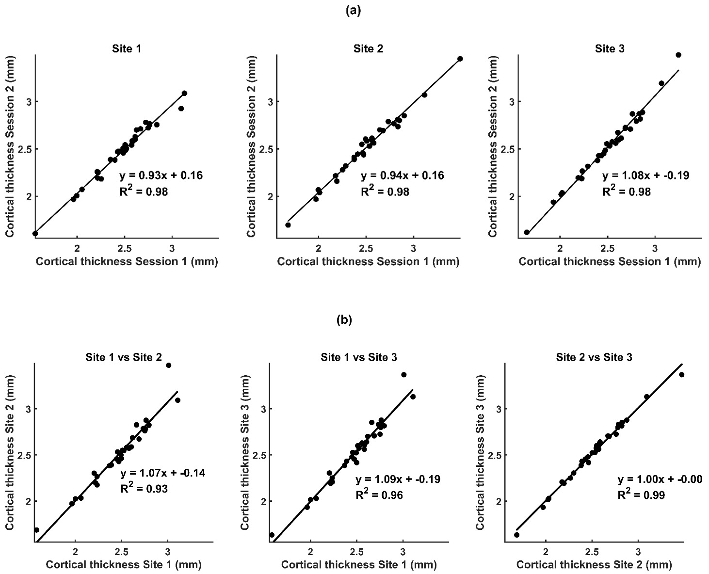
Cortical thickness measures were found to have excellent reproducibility (wCV% < 5%) and were strongly related (R² >0.90) across sessions and sites from our global measures, shown in Table 3 and Supplementary Table 1. When considering individual brain regions, as expected, greater variability was seen both within and between-sites (Supplementary Figures 1 and 2). The majority of ROIs interrogated showed a wCV% below 5% for cortical thickness when considering both within and between-sites. However, the entorhinal area showed an elevated wCV% of 7.2 % likely due to the location in the brain and the small volume of this region. When considering all ROIs together, the overall consistency (R² values) of measures across regions was high (R²>0.90) both within-sites (Table 4) and between-sites (Table 5), with no clear systematic biases, as shown by the gradient and/or intercept of the line of best fit from the linear regression (Figure 1).

Figure 1.Regression analysis of cortical thickness a) between-sessions at each site and b) between-sites. Each data point represents an ROI included in the analysis, names of each of the ROIs are given in Supplementary Figure 1.

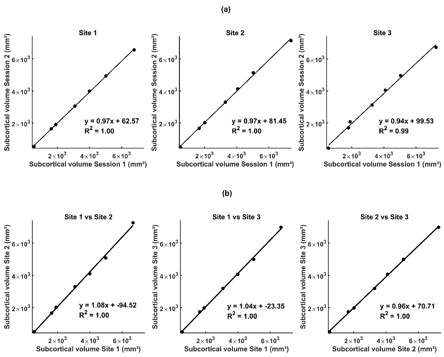
Regarding subcortical volumes, as expected due to the small volumes considered in many structures, the wCV% were in general larger than for the cortical thicknesses (Table 3 and Supplementary Table 1). When considering subcortical volumes (Table 3), the wCV% remained excellent (< 5%) showing high reproducibility. In general, for each ROI the wCV% both within and between-sites was also very good (<10%). The only exception was the nucleus accumbens where Site 3 had higher between scan variability (wCV% = 17.27%) which likely drove the between-site variability for this region (Supplementary Figures 3 and 4). Notably, the nucleus accumbens was the smallest volume measured (bottom left point on the graphs in Figure 2). Whilst the reproducibility of this structure was the lowest (Supplementary Table 1) it does sit on the line of best fit suggesting there is no systematic errors generated in measuring this volume within or between-sites. The overall consistency of measures from the linear regression across regions was excellent both within (Table 4 and Figure 2a) and between-sites (Table 5 and Figure 2b) with no clear systematic biases indicated by a change in the gradient and/or intercept of the line of best fit.

Figure 2.Regression analysis of subcortical volume a) between-sessions at each site b) between-sites. Each data point represents an ROI included in the analysis, names of each of the ROIs are given in Supplementary Figure 3.

These findings show the high reproducibility of structural measures of cortical thickness and subcortical volumes.

Fractional anisotropy and mean diffusivity

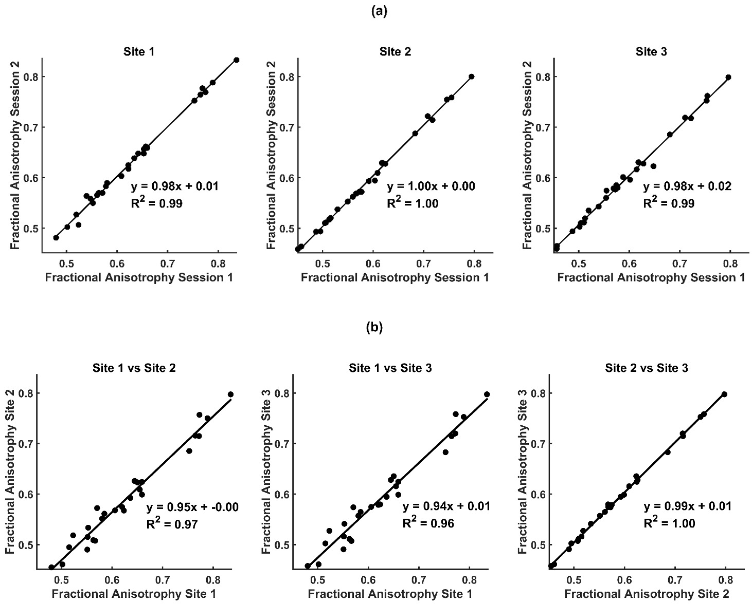
When considering white matter measures, FA exhibited excellent reproducibility (wCV% <5%) both across the whole brain white matter tracts (Tables 3 and Supplementary Table 1) and all regions included in the ROI analysis, within sites (Supplementary Figure 5) whilst very good reproducibility (wCV% <10%) of FA across sites within ROIS was achieved (Supplementary Figure 6). Figure 3 and Table 4 show that there was very good consistency in FA values across ROIs between-sessions within a site (high R², gradient close to 1 and intercept close to 0). However, there was some variation in values collected at Site 1 compared with Sites 2 and 3 (Figure 3b) which was likely to be driving the higher wCV% seen between-sites (Table 3 and Supplementary Figure 6).

Figure 3.Regression analysis of FA a) between-sessions at each site and b) between-sites. Each data point represents an ROI included in the analysis, names of each of the ROIs are given in Supplementary Figure 5.

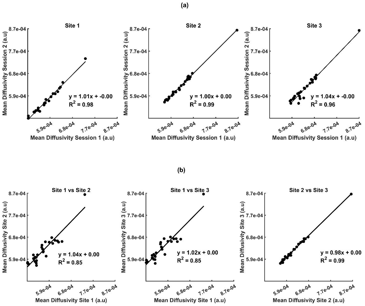
The MD measures showed a similar pattern of excellent reproducibility between-sessions within a site for the global measures and the average of all the ROI measures (wCV% <5%). Whilst very good reproducibility between-sites (wCV% <10%) was achieved for both the global measures (Table 3 and Supplementary Table 1) and individual ROIs (Supplementary Figures 7 and 8). Again, differences between Site 1 and Sites 2 and 3 clearly drove the lower reproducibility between-sites compared to within-site (Figure 4).

Figure 4.Regression analysis of a) MD between-sessions at each site and b) between-sites. Each data point represents an ROI included in the analysis, names of each of the ROIs are given in Supplementary Figure 7.

Together these findings show that excellent (within-site) and very high (between-site), reproducibility of FA and MD measures derived from our optimised DWI sequence were achieved.

Temporal signal to noise ratio

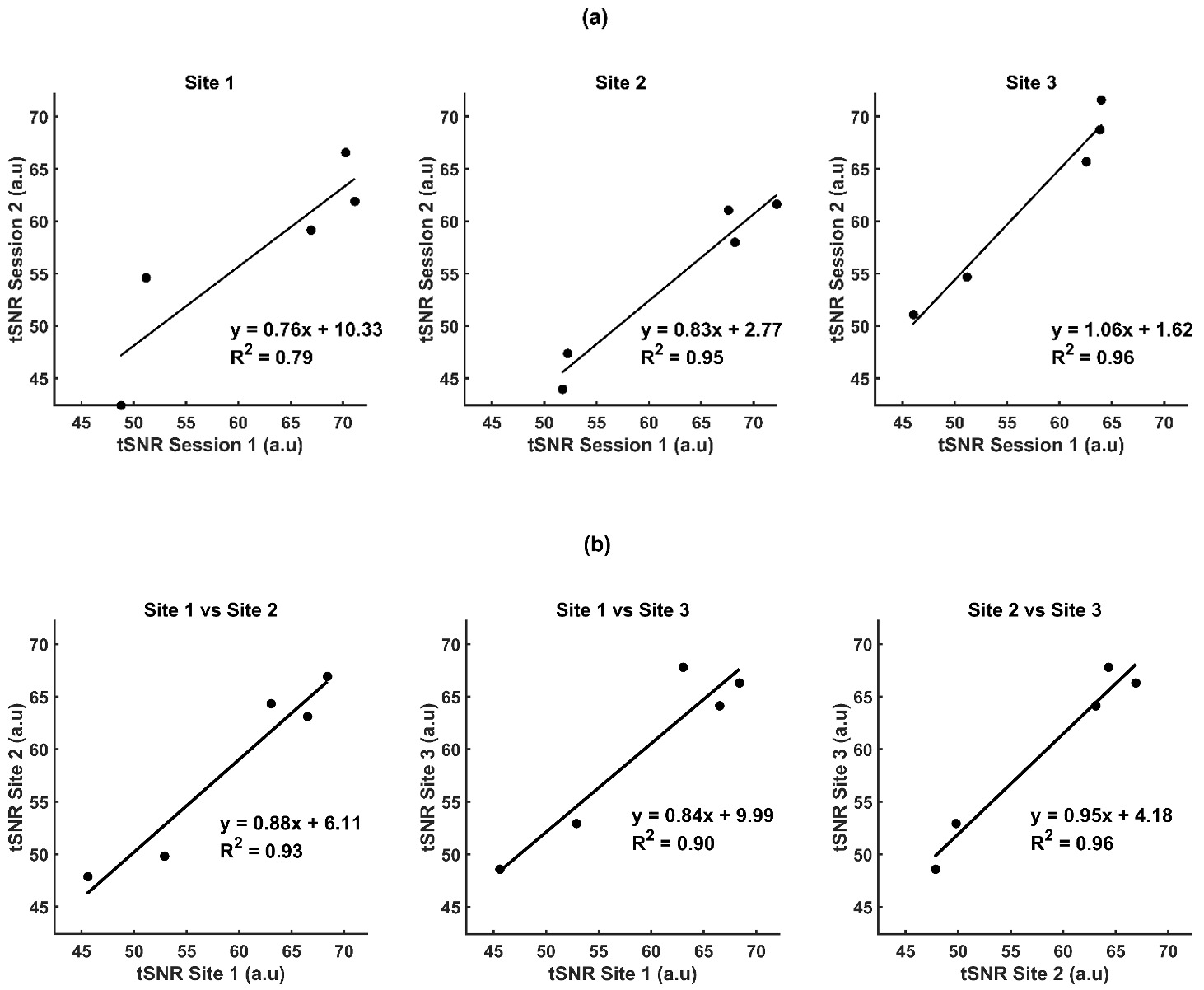
When considering tSNR across the whole of grey matter, in general we achieved excellent reproducibility both within-site and between-site (wCV%<5%, Table 3). The only exception to this was Site 2, where very good between session reproducibility was achieved (wCV%<10%, Table 3). When considering individual ROIs, there was a wider spread of values for the wCV% than seen in general for structural measures (Supplementary Figures 9 and 10). Mirroring the global values the between session reproducibility for individual ROIs was lowest (highest wCV% values) in Site 2 for the majority of regions considered, but a good reproducibility was reached in this site (wCV%<20%). When considering the consistency (R²) between-sessions across regions, Figure 5a shows that this was the lowest for Site 1 (lowest R², mostly driven by the two regions with the lowest tSNR, which were the frontal lobe and the occipital lobe). Figure 5b shows that between-sites, where values from the two within-site sessions had been averaged, the consistency across the ROIs was very high with R²>0.9.

Figure 5.Regression analysis of tSNR a) between-sessions at each site b) between-sites. Each data point represents an ROI included in the analysis, names of each of the ROIs are given in Supplementary Figure 9.

Cerebral blood flow

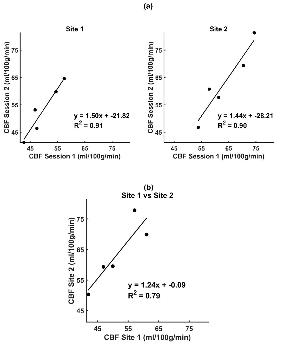
When assessing CBF across the entirety of grey matter, we observed within-site wCV% values <10%, indicating very good global CBF reproducibility. Notably, Site 1 exhibited higher wCV% values between the two sessions than Site 2, as shown in Table 3. Additionally, the between-site wCV% was <10%, reinforcing the overall very good reproducibility of this physiological measurement.

As expected, examination of individual ROIs revealed higher wCV% values compared to structural measures, as shown in Supplementary Figures 11 and 12. Interestingly, the regional variation in wCV% values was different for the two sites, with lower reproducibility in parietal and occipital lobes for Site 2, whilst the reproducibility was lower between-sessions in the motor and frontal lobes for Site 1 (Supplementary Figure 11). The between-session reproducibility was similar across sites for the cingulate gyrus, which interestingly had the lowest between-site reproducibility (Supplementary Figure 12). This between-site reproducibility was the lowest of all the measures considered in this work.

Despite the relatively low wCV% values (generally 10-20%) for each region, when considered over all the regions, the consistency (R²) between-sessions across these regions was very good for both Site 1 and Site 2, as indicated in Table 5 and Figure 6(a). However, in line with the reproducibility of the measures across regions between-sites, the between-site consistency was good but lower compared to all other between-site comparisons of MRI metrics made in this work, as illustrated in Figure 6(b).

Figure 6.Regression analysis of CBF a) between-sessions at each site b) between-sites. Each data point represents an ROI included in the analysis, names of each of the ROIs are given in Supplementary Figure 11.

Apparent point-spread function

For DWI, fMRI and pCASL data, the FWHM estimates were lower for the Philips system (Site 1) compared with the Siemens scanners (Sites 2 and 3), as shown in Supplementary Table 3. The magnitude of this difference between vendors varied between image acquisitions with the largest difference for fMRI data and the smallest for DWI data. Importantly, the largest differences in EES and TRT estimates between vendors were also seen in the fMRI acquisition (see Supplementary Table 3).

Motion parameters

DWI data

Motion estimates demonstrated higher overall total displacement at the Philips site (Site 1) compared with both Siemens sites (Sites 2 and 3). However, inspection of the motion parameters over time showed that the majority of the “motion” was linear drift due to heating of the gradient coils and passive shims which accumulated over time, due to the longer acquisition time at Site 1⁵⁴ (see Supplementary Figure 11). Looking at motion per unit time, the values were similar across sites, as expected (Supplementary Table 4). Importantly, all sessions remained well below the diffusion MRI motion thresholds (≈1 mm RMS; half-voxel criterion) generally considered acceptable for reliable tensor and fibre-tracking analysis.^55–57

fMRI data

Both framewise displacement and RMS values remained low across sessions and sites, with only a slight increase in motion observed during the first session at Site 2, RMS= 0.44±0.20 (mean ± SD) (see Supplementary Table 5). Overall, motion was small and did not vary systematically between sites.

pCASL data

Motion was minimal across sessions for these data. There was marginally higher fractional displacement observed in the Siemens site (Site 2, session 1) compared with all other sessions (see Supplementary Table 5). All sessions were below established thresholds for head motion (FD < 0.2 mm; RMS < 0.5 mm), consistent with accepted stability criteria for EPI-based acquisitions.^57,58

Discussion

Imaging techniques that yield consistent longitudinal measurements across different MRI scanners and vendors have become increasingly important as many clinical and neuroscience studies, including clinical trials, adopt multi-site approaches to data collection. The need for MRI metrics that are quantitative and reproducible across vendors, scanners and sites is vital for any measure that may become a clinically useful biomarker. Importantly, this is needed to move beyond the classical clinical use of MRI, which is to visually inspect and report on the structural images that are acquired in a clinical setting.⁵⁹ In this work, we investigated the reproducibility and consistency of MRI measures from optimised sequences and standard analysis pipelines with the view of using them to derive biomarkers for mTBI. Overall, motion remained low and stable across all sites, likely due to the considerable familiarity the participant had with the MRI environment. This low motion supported the subsequent between-site comparisons. The low levels of motion for this experienced participant suggest that the reproducibility between scanners of the sequences represents a best-case scenario; in patients, reproducibility is likely to be poorer. All of our measures at a global level exhibited at least very good reproducibility (wCV%<10%) with most of them categorised as excellent (wCV%<5%). The structural metrics were in general more reproducible and consistent than the measures derived from MR sequences designed to study aspects of brain function, as might be expected given the dynamic and integrative nature of brain function. Overall, we found excellent reproducibility (wCV%) and consistency (R²) between-sessions and sites for both the cortical thickness and subcortical volume measures. When considering individual regions all regions had at least very good (wCV% <10%) reproducibility. The highest wCV% (denoting poorest reproducibility) was in the entorhinal region for cortical thickness (Supplementary Figures 1 and 2) and nucleus accumbens for subcortical volume (Supplementary Figures 3 and 4). These regions are small and located near the inferior frontal portion of the brain, and prone to susceptibility artifacts due to the tissue-bone interface. These artifacts can make it challenging to accurately differentiate anatomical boundaries in these areas, potentially increasing the variability in cortical thickness and subcortical volume measurements.^36,37 However, despite these challenges we achieve very good reproducibility in these areas. Our results align with those of McGuire et al. (2017), Fujita et al. (2019) and Bano et al (2024) who reported poor reproducibility in the entorhinal region.^2,37,60 Similarly, the variation we observed in subcortical volume measurements in the nucleus accumbens area is generally consistent with other studies.^37,60 However, in general, these results show that we have successfully optimised our T1 anatomical sequence across scanners and vendors.

When considering the metrics derived from the DWI acquisition, FA and MD global measures showed excellent reproducibility both between and within-sites (Table 3). The wCV% values for FA within sites were considerably better than those reported in many other studies.^2,49,61 The mean global white matter FA between-sites achieved a wCV% <5%, similar to a multi-scanner study by Grech-Sollars and colleagues.⁶² The within-site reproducibility of the MD measures globally was still excellent (Table 3), but MD showed greater variability when measured in a number of specific white matter tracts (Supplementary Figures 7 and 8) compared with the FA values (Supplementary Figures 5 and 6). The reproducibility of MD between-sites was very good (showing wCV% 5 - 10%). Notably, the genu of the callosum exhibited a relatively higher between-site wCV%, but this remains below 10% indicating very good reproducibility between-sites. The overall pattern observed here, as well as the specific region with the highest wCV%, is in agreement with previous work.^51,63 While these results highlight the care that must be taken in interpreting metrics from different regions, in general they support the excellent reproducibility of DWI metrics.^60,61

When considering the between-site reproducibility specifically, it is clear that the reduction in reproducibility (R² values) that is seen for the MD and FA values compared with within-site values is driven by differences between-site 1 compared with Sites 2 and 3 (Figures 3 & 4b). Notably Site 1 had a Philips Ingenia scanner whilst Sites 2 and 3 both had a Siemens Prisma (Table 1). Although EES and TRT were well matched between vendors, differences in gradient performance and bore size could not be avoided. Vendor-related differences in diffusion timing, specifically the diffusion gradient separation time (Δ) and the diffusion gradient duration (δ), and readout characteristics were found with slightly longer values for the Philips system than the Siemens system, likely contributing to the observed variability.⁶⁴ Consistent with these vendor-related differences, the apparent point-spread function (FWHM) values were generally lower for the Philips system compared with the Siemens scanners, indicating sharper EPI spatial profiles across sessions for Philips DWI data. In addition, the Philips DWI sequence required a longer TR due to the hardware and safety constraints. The longer TR permits greater T₁ recovery between diffusion volumes, potentially altering baseline signal and SNR and introducing subtle inter-vendor bias in tensor fitting.^64,65 However, from our data we observed that the gradients and intercepts of the regression fits remain close to 1 and 0, respectively (Figures 3 and 4; Tables 4 and 5). Therefore, we suggest that the small between-vendor variability is unlikely to be driven by systematic differences between the systems but rather by subtle differences in SNR and acquisition characteristics driven by the differences in hardware.

A crucial property of EPI data, tSNR plays a vital role in ensuring reproducible results for any task performed during an fMRI acquisition. Therefore, to allow future fMRI results across scanners to be comparable, matching tSNR and ensuring it is as high as possible is important to assess during optimisation. Matching tSNR of EPI acquisitions across sites with different scanners is challenging due to several factors. tSNR will be affected by many facets of the MRI acquisition⁶⁶ from MRI hardware, pulse sequence design, to reconstruction methods e.g. parallel imaging techniques such as SENSE⁶⁷ vs GRAPPA⁶⁸ and multiband⁶⁹ implementations. In addition, EPI data will also be affected by physiological noise as well as the thermal noise that affects all MRI acquisition.^66,70 Therefore, reproducibility of tSNR between-sites is expected to be lower than within-site unless the scanners and sequences, to the level of the RF pulse designs, have been matched. This level of sequence matching between MR vendors is unfeasible in most studies and certainly not feasible within clinical settings where different hospitals have different 3T MRI scanners and CE/FDA markings must be maintained (i.e., altering pulse sequences and hardware would violate the CE marking).

With the known differences between scanners across sites (Table 1) in our study, we aimed to match tSNR as closely as possible. As outlined in the methods, this was done through an iterative process of altering multiband and image acceleration factors and assessing tSNR on a phantom (data not shown). This enabled us to match tSNR as closely as possible across sites whilst also maintaining matched TE, TR and voxel sizes, all crucial for fMRI studies. The optimised parameters are shown in Table 2, where at Site 1 MB = 2 with SENSE = 2 was used whereas at Sites 2 & 3 MB = 4 with no GRAPPA was used. Between vendor differences in the sequences were also reflected in the spatial smoothness metric: FWHM values were lower for the Philips site than the Siemens sites, mirroring the distinct echo-train durations and reconstruction methods used by each vendor. Previous work has shown that parallel imaging shortens the EPI echo train and reduces geometric distortion and T₂-related blurring, thereby yielding sharper spatial profiles.⁷¹ The differences in point-spread function that were seen may be overcome with post-processing smoothing of data, as previously suggested.⁷²

The wCV% and R2 of tSNR values when comparing between-sites indicate that the optimisation approach was largely successful in harmonising tSNR across scanners. Although small regional differences were present, when considering wCV across the three sites, between-site variability was comparable to, or slightly lower than, within-site variability, suggesting that between vendor optimisation was relatively successful. Importantly, the regression fits of between-site versus within-site tSNR values showed slopes close to unity and minimal intercept offsets, indicating the absence of systematic bias or directional differences between scanners. However, our analysis cannot eliminate the possibility of regional systematic differences. Together, these findings suggest that the optimisation reduced between-site differences in tSNR although some regional variability may still be present.

The optimisation we achieved produced lower variability than the ABCD study,² which scanned a single subject using four MRI scanners, and showed greater differences across sessions and sites than we observed. In our work, the variability (wCV%) was higher for the tSNR measures from the functional MRI than from the structural measures. This was expected due to the sensitivity of tSNR to physiological noise.⁷³ Large confounding factors that alter physiology such as caffeine⁷⁴ and nicotine⁷⁵ were minimised by the travelling head participant not consuming caffeine for 12 hours before and not smoking. Other factors such as time in the menstrual cycle⁷⁶ when scans were carried out was not controlled for, as this would not be typically controlled for in future work using these sequences. However, despite the physiological noise our results support previous work demonstrating that fMRI data quality results in very good reproducibility (wCV% <10%) and good consistency (R² >0.75) globally and therefore is reliable across sessions and sites.^23,77

CBF measures using ASL are inherently more difficult to match across sessions and scanners than many other MRI measures due to the low signal to noise ratio of the acquisition, combined with differences in sequences across vendors.⁷⁸ Like BOLD fMRI, subject motion, acquisition techniques, and post-processing errors can also contribute to small differences in CBF reproducibility.⁷⁹ We attempted to mitigate as many sources of variability as we could by employing a multi-delay pCASL sequence with a 2D-EPI readout across all sites. We wanted to employ a multi-delay sequence since it is possible that changes in microvasculature in mTBI patients may alter transit times in the patient group we are interested in.⁸⁰ We employed the same analysis pipeline on data from both sites considered.⁸¹ As a result of our approach, the CBF measurements showed a very good level of within-site reproducibility at both Site 1 and Site 2, as indicated by wCV% values<10% (Table 3). The slightly lower R² values between-sessions suggest decreased consistency within-sites compared with structural measures (Table 4), likely due to physiological variability.

When considering between-sites, our reliability was still very good (wCV% values<10%, Table 3) but of all the comparisons these were the lowest between-site agreement. In addition, the consistency when considering the different brain regions was lower with R²=0.795. This reflects the fact that these data were noisier and did not agree across sites as well as other measures. In addition, the estimated FWHM for pCASL images was considerably higher at the Siemens site than at the Philips site reflecting differences in EPI readout implementation and bandwidth contributed to variations in spatial smoothness (Supplementary Table 3). Our findings suggest for these CBF measures a larger change between groups will be needed to be detectable, compared with some of the other measures considered in this work, with inherently higher SNR. Nevertheless, these CBF variability observations agree with previous studies^78,82 and changes between groups in CBF measures have been reported.⁸³ The desire to have the multi-delay sequence and to match sequences across scanner platforms prevented the use of the recommended pCASL with 3D-GRASE readout sequence.⁸⁴ However, if this had been available to us at all sites, we would have opted for this sequence which is likely to have improved the reliability of the CBF results obtained, whilst retaining the capability for multi-delay.

Our results suggest the between-site variability is primarily attributed to differences in sequences and vendors across sites, rather than physiological factors which we would expect to observe in the within-site measures as well as the between-site measures. This interpretation is further supported by the minimal head motion observed across sessions (FD < 0.2 mm; RMS < 0.5 mm), indicating that motion-related effects were negligible. One study suggests that even minor changes in ASL sequences can significantly impact CBF measurement. Additionally, small variations in sequence parameters may have a larger effect on ASL reproducibility than hardware or software differences between vendors, even when the same labelling and readouts are used.⁸¹ The main differences in pCASL between the two sites are due to vendor-specific implementations. A more comprehensive comparison between vendors could be performed with additional subjects, given the slight differences in sequences. Moreover, factors like B0 field homogeneity and signal-to-noise ratio, which may not impact anatomical imaging, can significantly affect ASL sequences.⁸⁵ These findings highlight the inherent challenges of achieving consistent ASL CBF quantification across multiple MRI platforms. To improve reproducibility in future studies, additional steps such as vendor-specific calibration,⁸⁶ partial volume correction,⁸⁷ and post-acquisition harmonisation⁸⁸ may help to minimise systematic differences and enhance cross-site comparability. However, caution must be exercised when performing post-acquisition harmonisation as between group differences may be obscured if the region chosen to perform the harmonisation is unknowingly altered between the groups. For mTBI specifically this warrants further investigation in the future.

Limitations

Here we aimed to set up sequences for a subsequent assessment of variability of potential biomarkers of mTBI across a larger cohort of healthy controls and patients. A key limitation of this study is the use of a single healthy participant, which constrains both the choice of statistical analysis and statistical power. However, the primary aim was to examine the reproducibility of key imaging sequences across sessions and sites and to assess data quality prior to collecting data on a larger cohort involving both healthy and mTBI patients. This was a vital first step before progressing to a larger-scale variability study of 20 healthy participants and 20 with mTBI. This study focused specifically on acquisition-level protocol optimisation across scanners rather than applying post-acquisition statistical harmonisation methods. Our intention was to first evaluate the extent to which careful acquisition optimisation alone could minimise inter-scanner differences, thereby establishing a robust foundation for future harmonisation work. No post-acquisition pipelines were applied, and this should be considered when interpreting cross-site variability. This approach was chosen because improving similarity at the acquisition stage reduces the burden on post-acquisition harmonisation methods, which may not fully correct for vendor or sequence-dependent differences.²²

Additionally, the participant was a healthy adult female, whereas previous research suggests that the reproducibility of certain measures may be influenced by factors such as age and sex.^89,90 The study also did not control for the time of day at which the scans were acquired. However, the factors which cause variability due to time of day, point in menstrual cycle and sex is likely to be present and confounds in any study of clinical populations too.

Conclusion

This study assessed the reproducibility and consistency of multi-site imaging measurements, focussing on within and between-site differences using a single travelling head. We employed commonly used neuroimaging sequences in MRI, including T1, DTI, fMRI, and ASL, evaluating our ability to produce consistent results. Structural metrics exhibited excellent reproducibility across sessions and sites, while functional and physiological measures showed very good reproducibility between-sessions and sites, within the limits expected for measures from the human brain.⁴⁹ Overall, this study reports the reliability and reproducibility of neuroimaging measurements, demonstrating their value for evaluating biomarkers in mTBI and investigating disease status and treatment protocols.

Data and Code Availability

The imaging data used in this study are formatted according to the Brain Imaging Data Structure and stored on secure institutional servers. Although not publicly available at this time, the data will be made accessible via the OpenNeuro platform upon acceptance of the manuscript. The custom scripts used in the analysis are openly available on GitHub: https://github.com/MRIRW/mri-sequence-harmonisation.

Funding Sources

The work was funded by the Ministry of Defence, United Kingdom, through the mTBI Predict Consortium. The study was performed with the support of the Birmingham Clinical Trials Unit.

Ruwan Wanni Arachchige, Yidian Gao, Iman Idrees, Jessikah Fildes, Aliza Finch, and Waheeda Hawa, were all funded by the mTBI Predict Consortium at the time of data acquisition and analysis for this work.

Prof. Alexandra J. Sinclair is funded by a Sir Jules Thorn Award for Biomedical Science.

Conflicts of Interest

Professor Sinclair reports personal fees from Invex therapeutics in her role as Director with stock holdings, during the conduct of the study; other from Allergan, Novartis, Cheisi and Amgen outside the submitted work.

Acknowledgements

We acknowledge the input from the United Kingdom mTBI Predict Consortium.

This study has been delivered through the National Institute for Health and Care Research (NIHR) Birmingham Biomedical Research Centre (BRC). The views expressed are those of the author(s) and not necessarily those of the Ministry of Defence, United Kingdom, the NIHR or the Department of Health and Social Care.