Mass univariate aggregation methods for machine learning in neuroscience

Introduction

Machine learning serves as a crucial tool in neuroscience for enhancing our understanding of the human brain. The application of machine learning to neuroimaging data enables researchers to extract meaningful information from brain data and build predictive models that capture individual differences in brain-behavior relationships.^1,2 However, the high dimensionality of neuroimaging data, where the number of features often vastly outnumbers observations, presents significant analytical challenges.^1,3 Multiple machine learning methods that involve mass univariate regression followed by aggregation, which we term Mass Univariate Aggregation (MUA), have been introduced and demonstrated to be effective in high-dimensional data. Notably, because these methods evaluate each feature independently and yield an explicit, quantifiable measure of its contribution to the final score, they constitute a form of interpretable predictive modeling that enables direct identification of the brain connections driving a given prediction.^2,4

MUA methods represent a class of approaches that perform individual statistical tests on each feature separately (mass univariate), then combine weighted features into a unified predictive model (aggregation).^5–11 This philosophy underlies several successful methods across different fields. As an example, Polygenic Risk Scores (PRS), originally developed in genetics, aggregate the effects of individual genetic variants to predict complex traits and disease risk.^10–12 More recently, this approach was adapted from genetics to neuroimaging, introducing Polyconnectomic Scoring (PCS),^8,9 which generates an individual-level score reflecting the brain’s alignment with disorder- or behavior-related connectivity patterns. PCS computes this score using a previously derived connectome–symptom association matrix (referred to as the connectome summary statistics (CSS) matrix), which encodes the association between each brain connection and a specific disorder or behavioral phenotype, enabling assessment of new individuals’ connectivity patterns. Similarly, the Polyneuro Risk Scores (PNRS)⁷ utilizes a weighted aggregation of brain features to assess the generalizability of brain-behavior associations across independent samples; these aggregate scores can also be used in a final regression step, as demonstrated in recent applications of PNRS to ADHD symptom prediction.¹³ Additionally, Connectome-based Predictive Modeling (CPM)^5,6 is the most widely used MUA method in neuroimaging, employing binary feature selection based on statistical association, followed by sign-based aggregation of selected brain features and a final regression for behavioral prediction.

Although the core of the MUA algorithms is similar, their implementation remains fragmented across different programming languages and software platforms. CPM⁶ is primarily implemented in MATLAB with code from Yale,¹⁴ and a Python tutorial is also available from Finn,¹⁵ while PNRS⁷ is implemented in MATLAB with code from the Developmental Cognition and Neuroimaging (DCAN) lab at the University of Minnesota.¹⁶ PCS,^8,9 meanwhile, is available in MATLAB, Python, and R through the Dutch Connectome Lab.¹⁷ Moreover, the standard implementation for calculating PRS in genetics is provided by PRSice-2,^10,11 which is a C++ based software.

Here, we present a unified, open-source, and configurable pipeline that consolidates established mass univariate methods into a single platform compatible with modern machine learning workflows in Python. We validated the framework by reproducing results from previously published pipelines using the Human Connectome Project (HCP) dataset.¹⁸ Built within the scikit-learn architecture,¹⁹ this fully parametrized pipeline enables researchers to apply MUA approaches, including CPM,⁶ PNRS,⁷ and PCS^8,9 with support for both externally and internally derived CSS matrices, while leveraging the comprehensive scikit-learn ecosystem. Users can access the full range of cross-validation strategies, evaluation metrics, hyperparameter optimization tools, various regression methods, and pipeline variations that enable developers to extend and customize the framework according to their specific research needs.

By providing a unified platform for mass univariate aggregation methods, we aim to accelerate methodological development, reduce programming errors for researchers, and enhance reproducibility in brain-behavior prediction research.

Section 1. A Configurable Pipeline for Mass Univariate Aggregation Methods

Unified Configurable Pipeline Overview

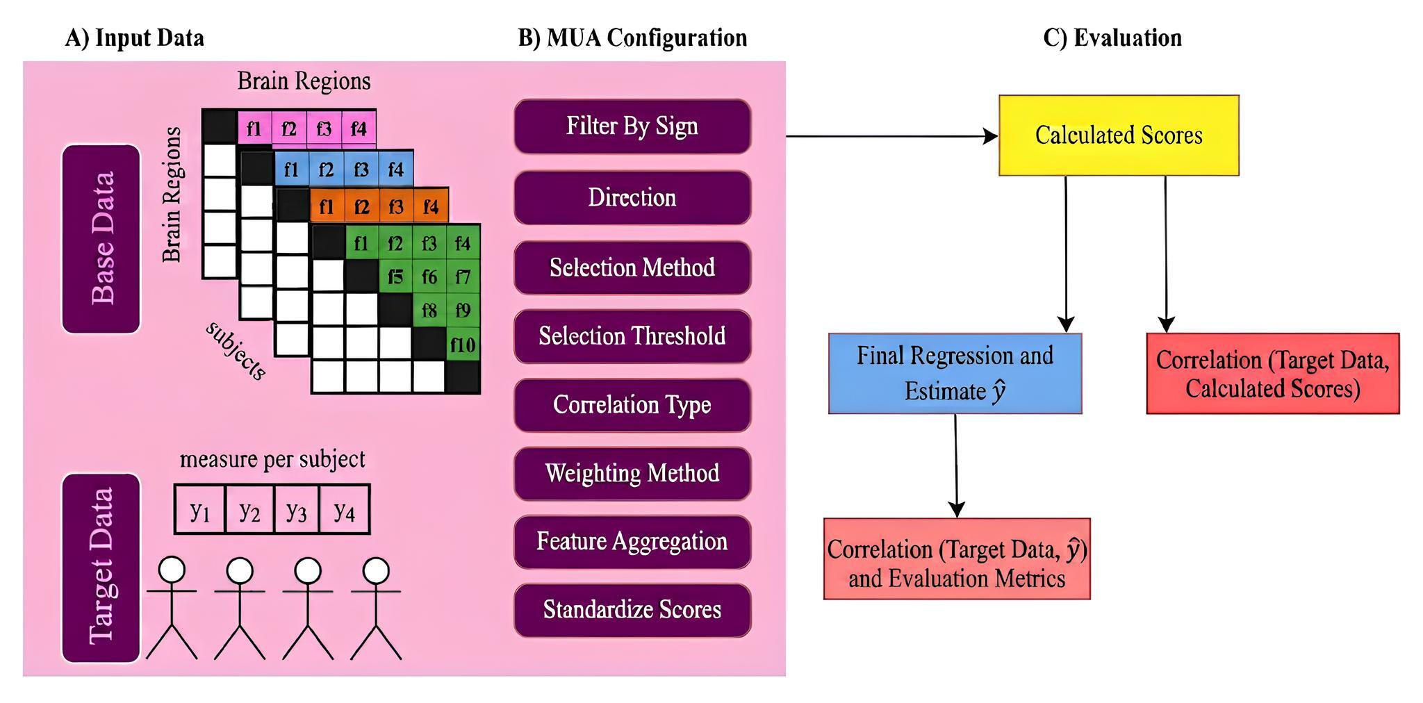
We developed a unified, configurable pipeline that integrates established methods, such as CPM⁶ and PNRS,⁷ alongside novel analytical approaches through a single interface (Figure 1). The pipeline is built around two core classes—FeatureVectorizer and MUA—both fully compatible with the scikit-learn ecosystem. These classes inherit from BaseEstimator and TransformerMixin, implementing the standard transformer interface (fit and transform) to ensure interoperability with Python’s machine learning infrastructure.

Figure 1.Overview of the unified configurable pipeline inputs and outputs for applying mass univariate aggregation methods. (A) Input data for the pipeline includes a matrix of features (n subjects × m predictors; e.g., edges from functional connectivity matrices) and a vector of observations (n subjects; e.g., behavioral measures). (B) The key parameters of the MUA class that are used for setting up the algorithm (for full descriptions of each parameter’s options, see Table 1). (C) The calculated scores can be evaluated in two ways: directly, by correlating scores with behavioral measures (cor(y, S)), or by adding a regression step to produce predictions and evaluating with correlation (cor(y, ŷ)) and diverse evaluation metrics (e.g., mean squared error).

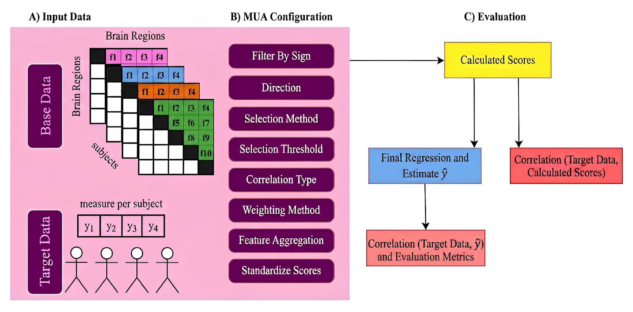
This modular architecture enables researchers to use standard scikit-learn features, including automated hyperparameter optimization via GridSearchCV and RandomizedSearchCV. The pipeline is model-agnostic and can incorporate any scikit-learn regression method. By adjusting parameters within this framework, researchers can reproduce existing methods, create hybrid approaches, or develop new strategies while leveraging scikit-learn’s comprehensive suite of cross-validation protocols (e.g., KFold, GroupKFold) and evaluation metrics (e.g., mean squared error, Pearson correlation).

Implementation Details

1. FeatureVectorizer Class

The FeatureVectorizer is designed to standardize symmetric graph input data for passing through the MUA class. When handling 3D connectivity input—represented as n subjects × m regions × m regions—it efficiently vectorizes the data by extracting only the off-diagonal upper triangular elements. If the input is already in a 2D feature format, the vectorizer leaves the data unmodified. Furthermore, the class supports inverse transformation, enabling the reconstruction of full symmetric matrices from feature vectors for subsequent usage. By streamlining these data transformations, our configurable pipeline can be used to apply MUA methods on neuroimaging data (connectivity matrices) and any other feature-outcome data.

2. MUA Class

The MUA class is our main Python class that extends scikit-learn’s BaseEstimator and TransformerMixin classes to ensure compatibility with standard machine learning pipelines; the MUA class operates through three steps:

I. Feature Selection: Determines which features are included based on their association with behavior (e.g., p-value thresholding, top-k selection, or all features).

II. Feature Weighting: Specifies how selected features are weighted (e.g., binary, correlation-based, or regression-derived weights).

III. Feature Aggregation: Defines how weighted features are combined into summary scores (e.g., sum or mean aggregation, with optional sign-based partitioning into positive and negative networks).

The MUA class employs a set of configurable parameters (Table 1) organized across the computational steps described above that enable flexible implementation of established methods while facilitating exploration of novel approaches.

The output of the MUA class is a 2D NumPy array of shape (n_samples, 1). When filter_by_sign is set to true, the class separately computes positive and negative network strengths and combines them according to the direction parameter — by default, as a difference score (aggregated positive network strength minus aggregated negative network strength), as popularized by the traditional CPM framework.⁶ Additionally, when filter_by_sign is set to false, all selected edges are processed together without sign-based partitioning and collapsed into a single weighted score, facilitating the implementation of the PCS^8,9 and PNRS⁷ methods.

3. Prediction Strategy

For methods such as PNRS,⁷ the aggregated score is used without a final regression step to produce a score that is correlated with, but not necessarily an actual prediction of, the outcome variable. As such, researchers typically use these scores as a new variable and observe their correlations with outcomes of interest, rather than using them as estimates of the outcome variable itself. Additionally, some approaches, such as CPM,⁶ include an additional step in which a final regression step is applied to the aggregated features to obtain a predicted value of the outcome variable. In both cases, after configuring the MUA class parameters, users can integrate any scikit-learn-compatible regression method directly into the pipeline via the ‘regressor’ step to estimate a final regression model using the aggregated features. The following section demonstrates the practical application of this approach (for further details, see CPM Configuration via The Configurable Pipeline, PNRS Configuration via The Configurable Pipeline, and Using PNRS as a Predictor with a Final Regression Step):

The_pipeline = Pipeline([

('vectorize', FeatureVectorizer()),

('mua', MUA(

...,

...,

)),

('regressor', LinearRegression()) # Linear regression

])

While LinearRegression() is used here as an example, the pipeline supports the integration of any alternative scikit-learn regression method, including custom implementations that follow the scikit-learn estimator interface.

4. Cross-Validation Strategy

For configurations that include a final regression step (e.g., CPM^6,14), predictions and performance estimates can be obtained using scikit-learn’s standard cross-validation utilities. Our pipeline supports any scikit-learn-compatible cross-validation splitter, including standard splitters (e.g., KFold) and group-aware splitters (e.g., GroupKFold). Note that the original CPM protocol employs k-fold cross-validation, which we demonstrate in Section 2 at the CPM Configuration via The Configurable Pipeline and use in Section 3 in our validation runs at the CPM Validation, but more generally, it is recommended to consider group-aware splitters whenever observations are non-independent — for example, in datasets with familial relationships such as HCP¹⁸ — to prevent data leakage and inflated performance estimates.^20,21 Users can specify the dependency structure through the groups argument (e.g., family ID), as demonstrated below (for further details and a full example, see Illustrative Application: Family-Aware Cross-Validation):

 # Load the family relationship data

 family_data = ...

 gkf = GroupKFold(n_splits=10)

 scores = cross_val_score(

 the_pipeline, brain_data, behavior,

 cv=gkf, groups=family_data

 )

 predictions = cross_val_predict(

 the_pipeline, brain_data, behavior,

 cv=gkf, groups=family_data

 )

While GroupKFold is used here as an example, users can substitute any scikit-learn cross-validation splitter that accommodates dependency structure, selecting the strategy best suited to their data and research design.

Section 2. Common Neuroimaging Algorithms and their Pipeline Configurations

Connectome-based Predictive Modeling (CPM)

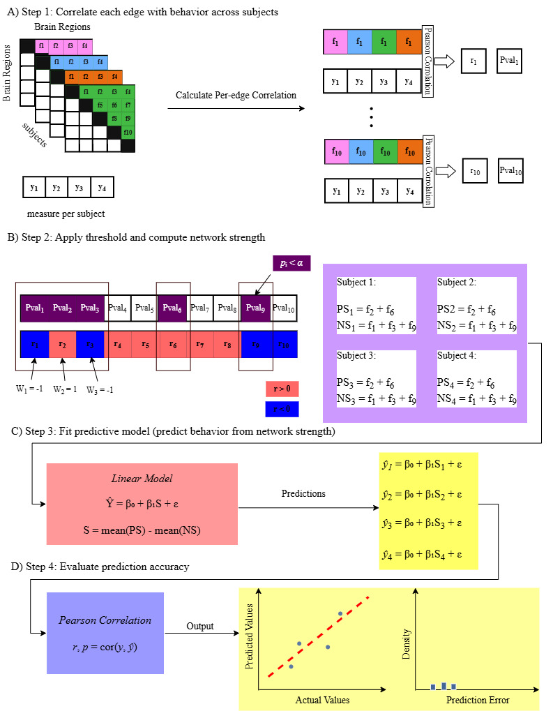
CPM⁶ identifies connectivity patterns that predict individual differences in behavior through sign-based aggregation (Figure 2).

Figure 2.Connectome-based Predictive Modeling (CPM) algorithm workflow. (A) For each subject (represented by a distinct color), a functional connectivity matrix is extracted, where each element represents the Pearson correlation between pairs of brain regions. Each feature (connectivity edge) is then correlated with the behavioral measure across subjects, yielding a correlation coefficient (r) and associated p-value per edge. (B) Edges are partitioned into positive (red) and negative (blue) networks according to the sign of their correlation with behavior. Edges are selected by applying a significance threshold (p < α). For each subject, a single summary score is computed as the difference between the mean connectivity of the positively and negatively correlated edges: S = mean(positive edges) − mean(negative edges). (C) A linear model uses the summary score to predict behavior (Ŷ = β₀ + β₁S + ε), generating individual predictions for each subject. (D) Model performance is assessed by correlating predicted and observed behavioral values. The scatter plot depicts prediction accuracy, with the dashed red line indicating the regression fit. The accompanying distribution of prediction errors illustrates variability in model performance across subjects.

The method consists of the following steps:

1. Feature Selection. Let X be the connectivity matrix with n subjects and m features, where x_ij represents the connectivity value for subject j and feature i. Let y be the behavioral measure vector for all subjects. For each connectivity feature i (where i = 1, …, m), compute the Pearson correlation coefficient r_i between feature vector x_i and behavioral measure y, along with its corresponding p-value p_i (Figure 2A). Then, given a significance threshold α, select features based on statistical significance:

\[S = \{ i:\ p_i < \ \alpha\}\ \]

where S is the set of indices for selected features.

2. Sign-Based Aggregation. Partition the selected features S into two subsets based on their correlation sign (Figure 2B):

\[S_{+}\ = \ \{ i\ \in \ S\ :\ r_i\ > \ 0\}\]

\[S_{-}\ = \ \{ i\ \in \ S\ :\ r_i\ < \ 0\}\]

This binary weighting approach assigns equal importance to all selected features regardless of their correlation magnitude.

3. Behavioral Prediction. Fit a linear model using a single summary score as the predictor, computed by taking the difference between the mean connectivity of positively and negatively correlated features (Figure 2C):

\[S_j\ = \ mean(X\lbrack S_{+},\ j\rbrack)\ - \ mean(X\lbrack S_{-},\ j\rbrack)\]

\[\hat{y}_j\ = \ \beta_0\ + \ \beta_1 S_j\]

where β₀ is the intercept and β₁ is the regression coefficient.

4. Evaluation. Assess the prediction accuracy by computing the Pearson correlation coefficient r and its associated p-value p (Figure 2D):

\[r,\ p\ = \ cor(y,\ \hat{y})\]

where \(y\) is the vector of actual behavioral values and \(\hat{y}\) is the vector of predicted values.

CPM Configuration via The Configurable Pipeline

The traditional CPM⁶ algorithm, following the Yale MATLAB implementation,¹⁴ can be implemented within our configurable pipeline using the RobustRegression() wrapper — a custom scikit-learn-compatible class available in our repository — with the following configuration:

cpm_pipeline = Pipeline([

('vectorize', FeatureVectorizer()),

('mua', MUA(

filter_by_sign=True,

direction='difference',

selection_method='pvalue',

selection_threshold=0.05,

weighting_method='binary',

feature_aggregation='mean',

)),

('regressor', RobustRegression()) # Robust regression

])

# Cross-validation

cpm_scores = cross_val_score(cpm_pipeline, brain_data, behavior, cv=10)

cpm_predictions = cross_val_predict(cpm_pipeline, brain_data, behavior, cv=10)

print(f"CPM R² (10-fold CV): {cpm_scores.mean():.3f} ± {cpm_scores.std():.3f}")

# Evaluation

cpm_r, cpm_p = pearsonr(behavior, cpm_predictions)

mae = mean_absolute_error(behavior, cpm_predictions)

rmse = np.sqrt(mean_squared_error(behavior, cpm_predictions))

r2 = r2_score(behavior, cpm_predictions)

The key parameters in the MUA class that define CPM⁶ are:

• filter_by_sign=True creates separate positive and negative network scores

• direction='difference' computes a single summary score as (positive network score – negative network score)

• selection_method='pvalue' with threshold=0.05 implements statistical feature selection

• weighting_method='binary' assigns equal weights to all selected features (connectivity edge)

• feature_aggregation='mean' computes (mean(positive network score) – mean(negative network score))

The final prediction step uses a linear model, consistent with the CPM protocol description.⁶ Users can specify their preferred regression method via the ‘regressor’ step in the pipeline. For users who wish to use robust regression as their final prediction step, following the Yale MATLAB implementation,¹⁴ our repository provides a custom scikit-learn-compatible wrapper, called RobustRegression(), that closely replicates MATLAB’s robustfit (for further details, see CPM Validation and Limitations). Alternatively, users who prefer ordinary least squares, as in the Python CPM tutorial by Finn,¹⁵ can use scikit-learn’s LinearRegression(). More broadly, our pipeline supports any scikit-learn-compatible regression method, and users can also implement custom scikit-learn-compatible wrappers for additional regression approaches.

Polyneuro Risk Scores (PNRS)

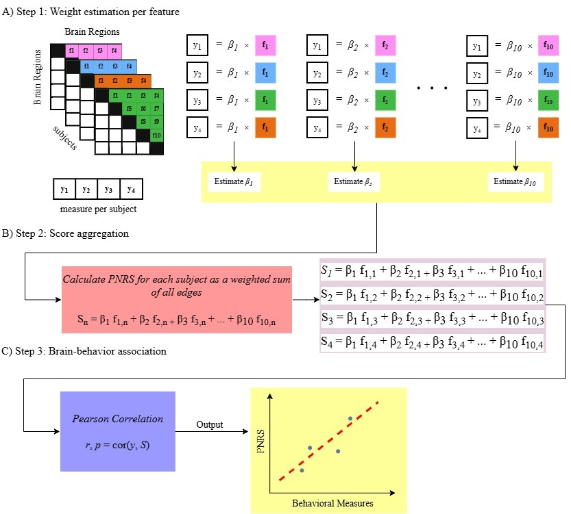
PNRS⁷ assesses brain-behavior associations through weighted aggregation, where each feature (connectivity edge) contributes proportionally to its univariate association strength (Figure 3).

Figure 3.Polyneuro Risk Scores (PNRS) methodology. (A) Functional connectivity matrices are extracted for each subject (represented by a distinct color). Each matrix contains connectivity values for all brain region pairs. For each connectivity edge (feature), a univariate regression coefficient (β weight) is estimated across subjects using the model \(y\ = \ \beta_i\ x_i\), where \(\beta_i\ = \ (x_i^Ty)\ /\ (x_i^Tx_i)\), yielding one β weight per edge (shown here for features f₁ through f₁₀). (B) For each subject j, the PNRS is computed as the weighted sum of all connectivity edges, where each edge is multiplied by its corresponding β weight (\(S_j\ = \ \beta_1 f_{1,j}\ + \ \beta_2 f_{2,j}\ + \ ...\ + \ \beta_{10} f_{10,j}\)). (C) The aggregated PNRS scores are correlated with the observed behavioral measures. The correlation coefficient r and its associated p-value quantify the strength of the brain-behavior association captured by the score.

The method consists of the following steps:

1. Feature Selection. Let X be the connectivity matrix with n subjects and m features, where x_ij represents the connectivity value for subject j and feature i. Let y be the behavioral measure vector for all subjects (Figure 3A).

All m connectivity features are retained and for each feature i (where i = 1, …, m), the univariate regression coefficient β_i will be computed:

\[y\ = \ \beta_i\ x_i\]

where x_i is the vector of connectivity values for feature i across all subjects, and the coefficient is computed as:

\[\beta_i\ = \ (x_i^Ty)\ /\ (x_i^Tx_i)\]

2. Score Aggregation. For each subject j, compute a single aggregated score S_j by summing all features weighted by their regression coefficients (Figure 3B):

\[S_j\ = \ \sum_{i\ = \ 1}^{m}{\beta_i\ x_{ij}}\]

This creates a composite score that reflects the cumulative effect of all brain features.

3. Evaluation. Assess the strength of the brain-behavior association by computing the Pearson correlation coefficient r and its associated p-value p between the aggregated scores and the behavioral measure (Figure 3C):

\[r,\ p\ = \ cor(y,\ S)\]

where r quantifies the strength of the linear association between the brain-wide connectivity pattern and the behavioral measure.

PNRS Configuration via The Configurable Pipeline

The PNRS⁷ algorithm, used for in-sample validation against the BWAS MATLAB toolbox¹⁶ can be implemented within our configurable pipeline using the following configuration. This configuration uses all connectivity features without selection, creating a comprehensive brain-wide score.

pnrs_pipeline = Pipeline([

('vectorize', FeatureVectorizer()),

('mua', MUA(

filter_by_sign=False,

selection_method='all',

weighting_method='regression',

feature_aggregation='sum',

))

])

pnrs_scores = pnrs_pipeline.fit_transform(brain_data, behavior)

# Evaluation

pnrs_r, pnrs_p = pearsonr(behavior, pnrs_scores.flatten())

The key parameters in the MUA class that define PNRS⁷ are:

• filter_by_sign=False processes all features (connectivity edges) together without sign-based partitioning into positive and negative networks.

• selection_method='all' includes every feature without statistical thresholding

• weighting_method='regression' assigns beta weights from univariate regressions (\(\beta_i\ = \ (x_i^Ty)\ /\ (x_i^Tx_i)\))

• feature_aggregation='sum' computes the score as a weighted sum of all features

Using PNRS as a Predictor with a Final Regression Step

The PNRS⁷ pipeline can also be adapted to accommodate a final regression step.¹³ We are unable to validate this exact version of the pipeline since it has not been previously released to our knowledge; however, the individual components — the PNRS computation and the final regression step — are each independently validated through the original PNRS and the CPM⁶ pipeline. This configuration is as follows:

pnrs_pipeline = Pipeline([

('vectorize', FeatureVectorizer()),

('mua', MUA(

filter_by_sign=False,

selection_method='all',

weighting_method='regression',

feature_aggregation='sum',

)),

('regressor', LinearRegression()) # Linear regression

])

# Cross-validation

pnrs_scores = cross_val_score(pnrs_pipeline, brain_data, behavior, cv=10)

pnrs_predictions = cross_val_predict(pnrs_pipeline, brain_data, behavior, cv=10)

print(f"PNRS R² (10-fold CV): {pnrs_scores.mean():.3f} ± {pnrs_scores.std():.3f}")

# Evaluation

pnrs_r, pnrs_p = pearsonr(behavior, pnrs_predictions)

mae = mean_absolute_error(behavior, pnrs_predictions)

rmse = np.sqrt(mean_squared_error(behavior, pnrs_predictions))

r2 = r2_score(behavior, pnrs_predictions)

The key parameters in the MUA class that define PNRS⁷ with final regression are as above with the exception of the additional parameter ‘regressor’ set to LinearRegression().

Polyconnectomic Scoring (PCS)

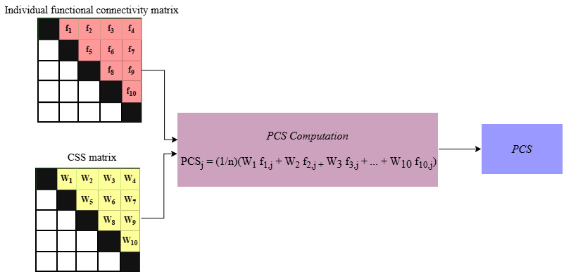
PCS^8,9 measures how similar an individual’s brain functional connectivity pattern is to the connectivity pattern associated with a specific disorder or behavior (Figure 4). To compute this score, researchers first estimate CSS using large discovery datasets. These statistics quantify the association between each functional connection and the disorder or behavior (specifically, regression coefficients for scale variables, analogous to the regression-derived weights used in the PNRS⁷ framework to assess brain-behavior associations, and Cohen’s d for group contrasts). The resulting CSS values form a matrix of edge-wise weights representing the disorder- or behavior-related connectivity pattern (Figure 4, CSS matrix). The PCS for a new individual (Figure 4, individual functional connectivity matrix) is then computed by aggregating their functional connectivity values weighted by the corresponding CSS values, producing a score that reflects how strongly the individual’s connectome resembles the disorder- or behavior-associated connectivity pattern.

\[{PCS}_{j}\ = \ \frac{1}{n}\ \sum_{e\ = \ 1}^{n}{{FC}_{j,e}\ \times \ {CSS}_{e}}\]

where FC_j,e denotes the functional connectivity value of edge e for subject j, CSS_e represents the connectome summary statistic for edge e, and n is the total number of connections included in the score.

Figure 4.Polyconnectomic Scoring (PCS) methodology. An individual’s functional connectivity matrix (top left, pink) contains connectivity values (f₁ through f₁₀) and a connectome summary statistic (CSS) matrix (bottom left, yellow) contains pre-computed edge-wise weights (W₁ through W₁₀) derived from a large discovery dataset, where each weight quantifies the association between a given connectivity edge and the disorder or behavioral measure of interest. The PCS is computed as the weighted mean of the individual’s connectivity values multiplied by their corresponding CSS weights: \(\scriptsize PCS_j\ = \ \frac{1}{10}(W_{1}f_{1,j}\ + \ W_{2}f_{2,j}\ + \ W_{3}f_{3,j}\ + \ ...\ + \ W_{10}f_{10,j})\). The resulting PCS (right) provides a single scalar index reflecting the degree to which the individual’s connectivity pattern resembles the disorder-associated connectivity profile.

PCS Configuration via the Configurable Pipeline

Because of the shared computational backbone of MUA methods, our pipeline naturally accommodates PCS^8,9 analyses: users supply a pre-computed CSS vector as external weights, and PCS is produced within the same analytical workflow used for other MUA approaches. The pipeline accepts any array-like structure as CSS (e.g., NumPy array, Python list, or Pandas Series), provided as a one-dimensional vector of edge-wise weights whose length equals the number of unique edges in the upper triangle of the connectivity matrix. When the CSS is available as a full regions × regions matrix, the upper triangle can be extracted via np.triu_indices(n, k=1) to produce the required vector format for the pipeline. FeatureVectorizer is included in the pipeline to apply the same extraction to the input connectivity matrices, ensuring consistent edge ordering between the CSS and the data:

# Load pre-computed CSS matrix from discovery study CSS_matrix = ...

# Extract upper triangle to match vectorized FC edges

CSS = CSS_matrix[np.triu_indices(n_nodes, k=1)]

pcs_pipeline = Pipeline([

('vectorize', FeatureVectorizer()),

('mua', MUA(

filter_by_sign=False,

selection_method='all',

weighting_method='external',

external_weights=CSS,

feature_aggregation='mean',

))

])

pcs_scores = pcs_pipeline.fit_transform(brain_data, behavior)

pcs_results = pcs_scores.flatten()

The key parameters in the MUA class that define PCS^8,9 are:

• filter_by_sign=False processes all features (connectivity edges) together without sign-based partitioning into positive and negative networks.

• selection_method='all' includes every feature, consistent with the application of a full CSS weight map.

• weighting_method='external' with external_weights applies an externally derived CSS containing edge-wise weights associated with a specific disorder or behavioral phenotype

• feature_aggregation='mean' computes the PCS value as the average weighted connectivity across all features

Computing CSS Within the Pipeline

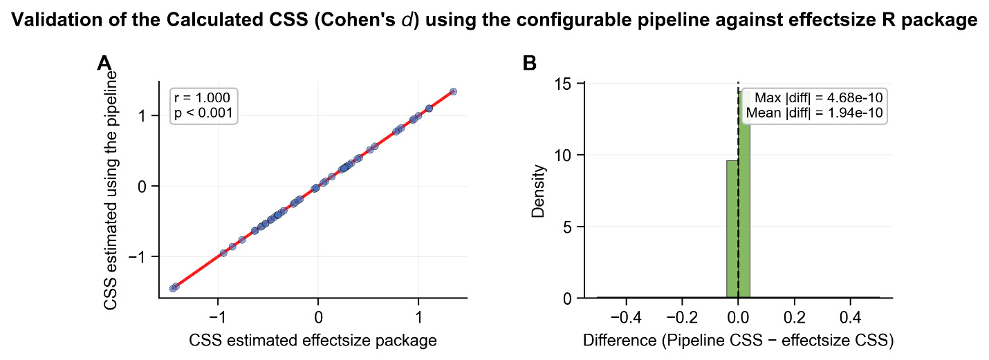
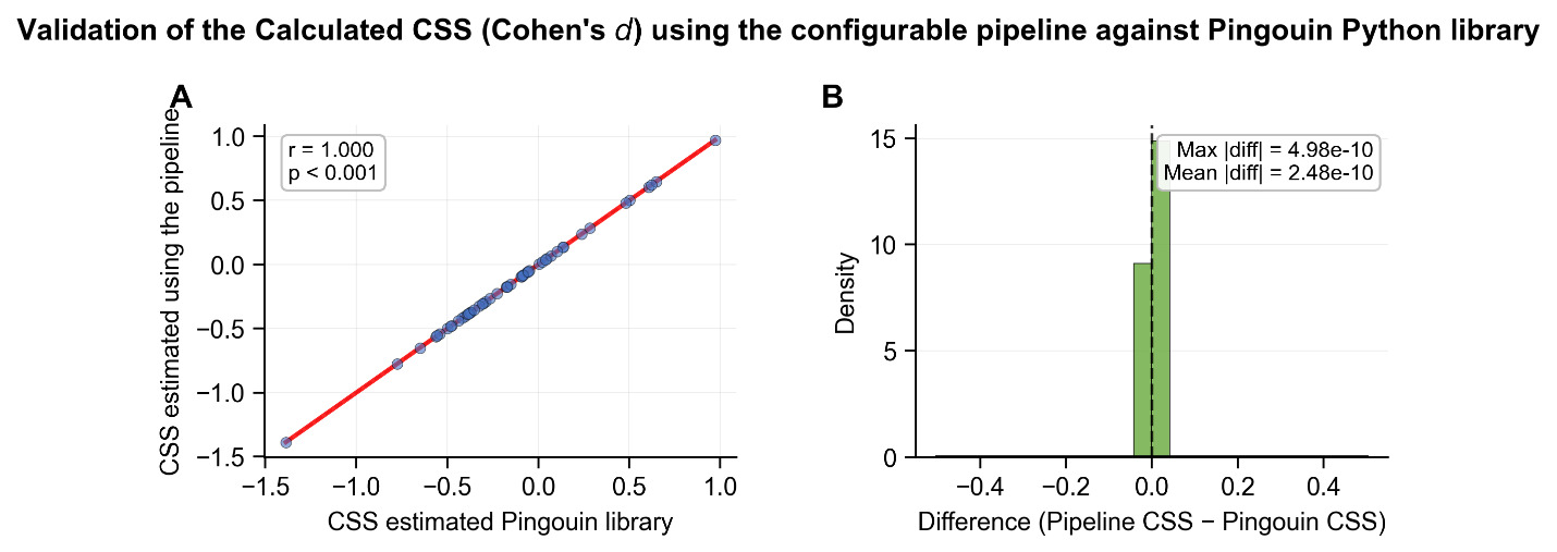
Beyond applying pre-computed CSS, users can use our pipeline to derive CSS from a discovery sample. For scale variables, CSS can be extracted as univariate regression coefficients (β-weights). For group contrasts, CSS is expressed as Cohen’s d.^8,9 Our pipeline supports this by first computing edge-wise correlations from the discovery sample and then converting them to Cohen’s d using established formulas derived either directly or through the t-statistic.^22–24 Our implementation uses the t-statistic-based conversion, as this enabled validation against the effectsize R package,^25,26 which implements the same approach; to our knowledge, no existing study implements the direct correlation-to-Cohen’s d conversion formula. Alternatively, users can compute Cohen’s d externally using dedicated tools in Python (e.g., the Pingouin²⁷ Python library), which compute Cohen’s d from the means and standard deviations of the two groups.²⁸ All three approaches — direct computation from group statistics, and the two correlation-to-Cohen’s d conversions — are presented in Appendix A.

Note that the pipeline’s built-in correlation-to-Cohen’s d conversion computes unadjusted effect sizes for two-group contrasts; however, CSS matrices from prior PCS studies have sometimes been derived using Cohen’s d corrected for covariates such as age, sex, and in-scanner motion.^8,9 For datasets requiring confound correction, multi-group contrasts, or other custom CSS for PCS computations, users can derive weights externally and supply them via the external_weights parameter.

The pipeline computes and stores CSS internally as a one-dimensional vector. To save the resulting CSS as a full regions × regions matrix, users can reconstruct it using FeatureVectorizer.inverse_transform.

1. Scale Variables

For scale variables (e.g., fluid intelligence), CSS is computed as univariate regression coefficients.^8,9 Users can derive these weights from a discovery sample and apply them as external weights to compute PCS in a validation sample. As there is no publicly available CSS implementation from prior studies to validate against, we were unable to validate this CSS derivation step directly. Since the CSS values for scale variables are mathematically identical to the regression coefficients used in PNRS⁷ (both computed as \(\beta_i\ = \ (x_i^Ty)\ /\ (x_i^Tx_i)\)), our validated PNRS implementation confirms the correctness of this step.

 # Step 1: Derive CSS (β-weights) from discovery sample

 css_pipeline = Pipeline([

 ('vectorize', FeatureVectorizer()),

 ('mua', MUA(

 filter_by_sign=False,

 selection_method='all',

 weighting_method='regression',

 feature_aggregation='sum',

 ))

 ])

 css_pipeline.fit(brain_data_discovery, behavior_discovery)

 CSS = css_pipeline.named_steps['mua'].edge_weights_

 # Save CSS as a symmetric matrix CSV

 vectorizer = css_pipeline.named_steps['vectorize']

 CSS_matrix = vectorizer.inverse_transform(

 CSS.reshape(1, -1))[0]

 pd.DataFrame(

 CSS_matrix,

 index=region_labels, columns= region_labels

 ).to_csv('css_beta_weights.csv')

 # Step 2: Apply CSS to compute PCS in validation sample

 pcs_pipeline = Pipeline([

 ('vectorize', FeatureVectorizer()),

 ('mua', MUA(

 filter_by_sign=False,

 selection_method='all',

 weighting_method='external',

 external_weights=CSS,

 feature_aggregation='mean',

 ))

 ])

 pcs_scores = pcs_pipeline.fit_transform(brain_data_validation, behavior_validation)

 pcs_results = pcs_scores.flatten()

2. Group Contrasts

For two-group contrasts (e.g., patients vs. controls), CSS is expressed as Cohen’s d.^8,9 Users can use our configurable pipeline to derive edge-wise correlations between connectivity values and binary group labels from a discovery sample and convert them to Cohen’s d .^22–24 When binary group labels are provided (e.g., 0 = controls, 1 = patients), the resulting Pearson correlations are mathematically equivalent to point-biserial correlations, which can be directly converted to Cohen’s d without additional configuration.

\[\small d_e\ = \ \frac{r_{e}}{\sqrt{\left( 1 - r_{e}^{2}\, \right)}}\ \times \ \sqrt{(\frac{{(n}_{1} + n_{2}\ - \ 2)\ }{n_{1}} + \frac{{(n}_{1} + n_{2}\ - \ 2)\ }{n_{2}})}\]

where r_e is the correlation for edge e, and n₁ and n₂ are the sample sizes of the two groups. This equation is derived through the t-statistic,^23,24 which is also used in the effectsize R package.^25,26 Full derivations are provided in Appendix A.

 # Step 1: Derive correlations from discovery sample

 css_pipeline = Pipeline([

 ('vectorize', FeatureVectorizer()),

 ('mua', MUA(

 filter_by_sign=False,

 selection_method='all',

 weighting_method='correlation',

 feature_aggregation='sum',

 ))

 ])

 css_pipeline.fit(brain_data_discovery, group_labels_discovery)

 r = css_pipeline.named_steps['mua'].correlations_

 # Convert correlation to Cohen's d (general formula)

 n1 = np.sum(group_labels_discovery == 0) # e.g., controls

 n2 = np.sum(group_labels_discovery == 1) # e.g., patients

 # Correlation-to-Cohen's d conversion

 CSS_cohen_d = (r / np.sqrt(1 - r**2)) * np.sqrt(

 ((n1 + n2 - 2) / n1) + ((n1 + n2 - 2) / n2)

 )

 # Save CSS as a symmetric matrix CSV

 vectorizer = css_pipeline.named_steps['vectorize']

 CSS_cohen_d_matrix = vectorizer.inverse_transform(

 CSS_cohen_d.reshape(1, -1))[0]

 pd.DataFrame(

 CSS_cohen_d_matrix,

 index=region_labels, columns= region_labels

 ).to_csv('css_cohen_d.csv')

 # Step 2: Apply CSS to compute PCS in validation sample

 pcs_pipeline = Pipeline([

 ('vectorize', FeatureVectorizer()),

 ('mua', MUA(

 filter_by_sign=False,

 selection_method='all',

 weighting_method='external',

 external_weights=CSS_cohen_d,

 feature_aggregation='mean',

 ))

 ])

 pcs_scores = pcs_pipeline.fit_transform(brain_data_validation, group_labels_validation)

 pcs_results = pcs_scores.flatten()

Section 3. Validation

To ensure the accuracy of our pipeline, we compared the results of our pipeline configurations for CPM⁶ and PNRS⁷ against their established MATLAB implementations^14,16 using the HCP data.¹⁸ The CPM protocol describes the final prediction step as a linear model, which has been implemented as robust regression in the Yale MATLAB code and as ordinary least squares in the Python CPM tutorial by Finn.¹⁵ Using identical fold assignments, we validated our pipeline against the Yale MATLAB implementation in two ways: (1) using our custom scikit-learn-compatible robust regression wrapper to closely replicate MATLAB’s robustfit, achieving near-perfect numerical equivalence on the HCP data; and (2) using scikit-learn’s LinearRegression, which, as expected in a large-sample single-predictor setting, showed high agreement, with residual differences reflecting the methodological distinction between ordinary least squares and robust regression rather than any pipeline error (for further details, see CPM Validation and Limitations). For PNRS, the pipeline achieved exact numerical equivalence. For PCS,^8,9 we validated two aspects of our pipeline. (1) PCS computation: To ensure that our pipeline correctly computes PCS, we compared its output against results obtained directly from the PCS formula. For this, we used the HCP data, consistent with the CPM and PNRS validations, alongside a simulated CSS matrix. (2) CSS computation for group contrasts (correlation-to-Cohen’s d conversion): To verify the pipeline’s correlation-to-Cohen’s d conversion,^22–24 we validated our results against the effectsize R package,^25,26 which implements the same r-to-d conversion derived from the t-statistic,^23,24 and independently against the Pingouin Python library, which uses the means and standard deviations of the two groups.²⁷ Both the PCS^8,9 computation and the CSS derivation approach matched exactly with their ground-truth values, confirming the correctness of our pipeline’s PCS computation and the correlation-to-Cohen’s d conversion via the t-statistic.^23,24

Complete validation scripts and visualization utilities for generating publication-quality figures of prediction accuracy and error distributions are available in the repository.

Additionally, to provide guidance on computational feasibility, we report single-run runtimes for each pipeline configuration, measuring only the core pipeline computation — excluding data loading and visualization — on a single CPU core (Intel Core i7, 10th generation, 8GB RAM; Table 2).

Dataset

We validated these pipelines using resting-state fMRI data obtained from the HCP.¹⁸ The dataset comprised 1067 subjects. Functional connectivity matrices were derived by preprocessing the data using the Yale preprocessing and functional connectivity estimation pipelines (cf. Noble et al.²⁹) to obtain resting-state functional connectivity data as the Pearson correlations between time series for each region of the Shen268 atlas,³⁰ yielding 268 × 268 symmetric matrices per subject. Following the original CPM,⁶ fluid intelligence scores served as the behavioral prediction target.

CPM Validation

We benchmarked our CPM implementation against the original Yale code^6,14 using HCP¹⁸ connectivity data (n = 1067) with a significance threshold of 0.05 and identical 10-fold cross-validation fold assignments to isolate algorithmic differences. As the original MATLAB implementation uses robust regression (robustfit) for the final prediction step, we created a scikit-learn-compatible wrapper available in the repository that uses statsmodels’ RLM³¹ with Tukey’s bisquare weighting to closely match this behavior, as no existing Python package exactly replicates MATLAB’s robustfit.

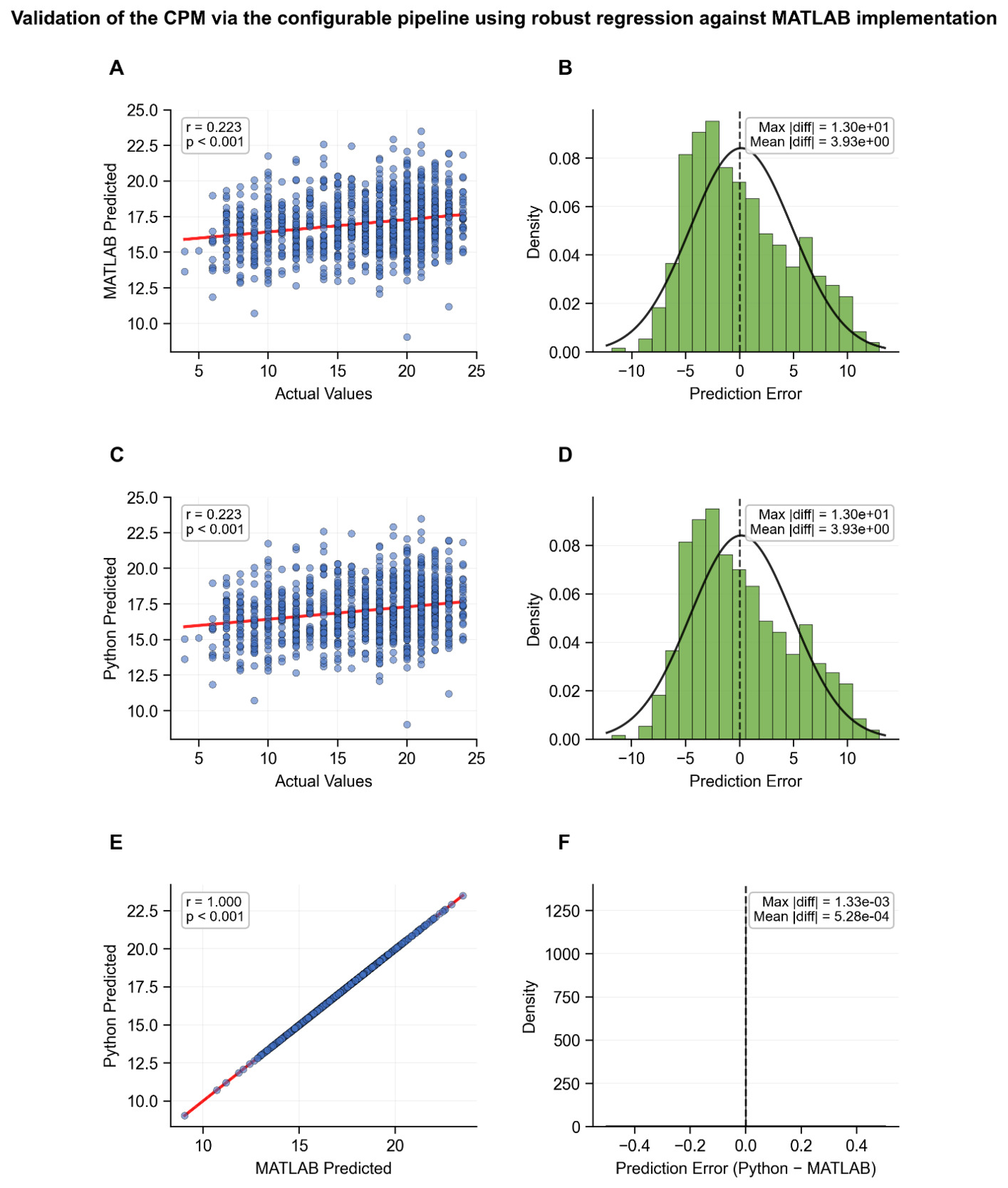
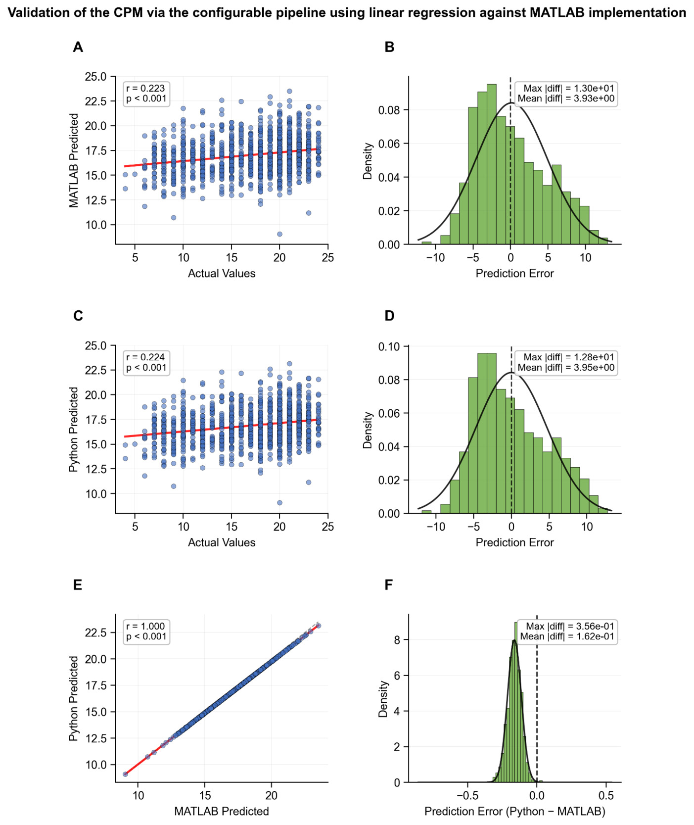
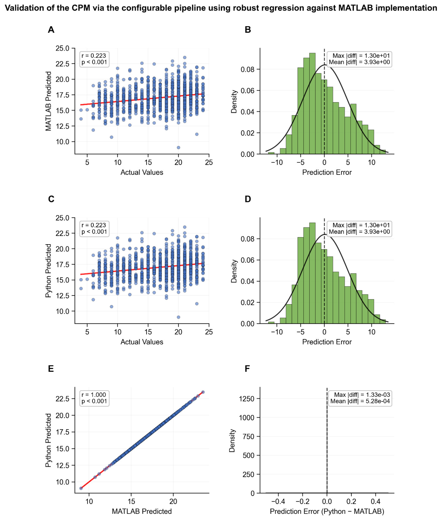
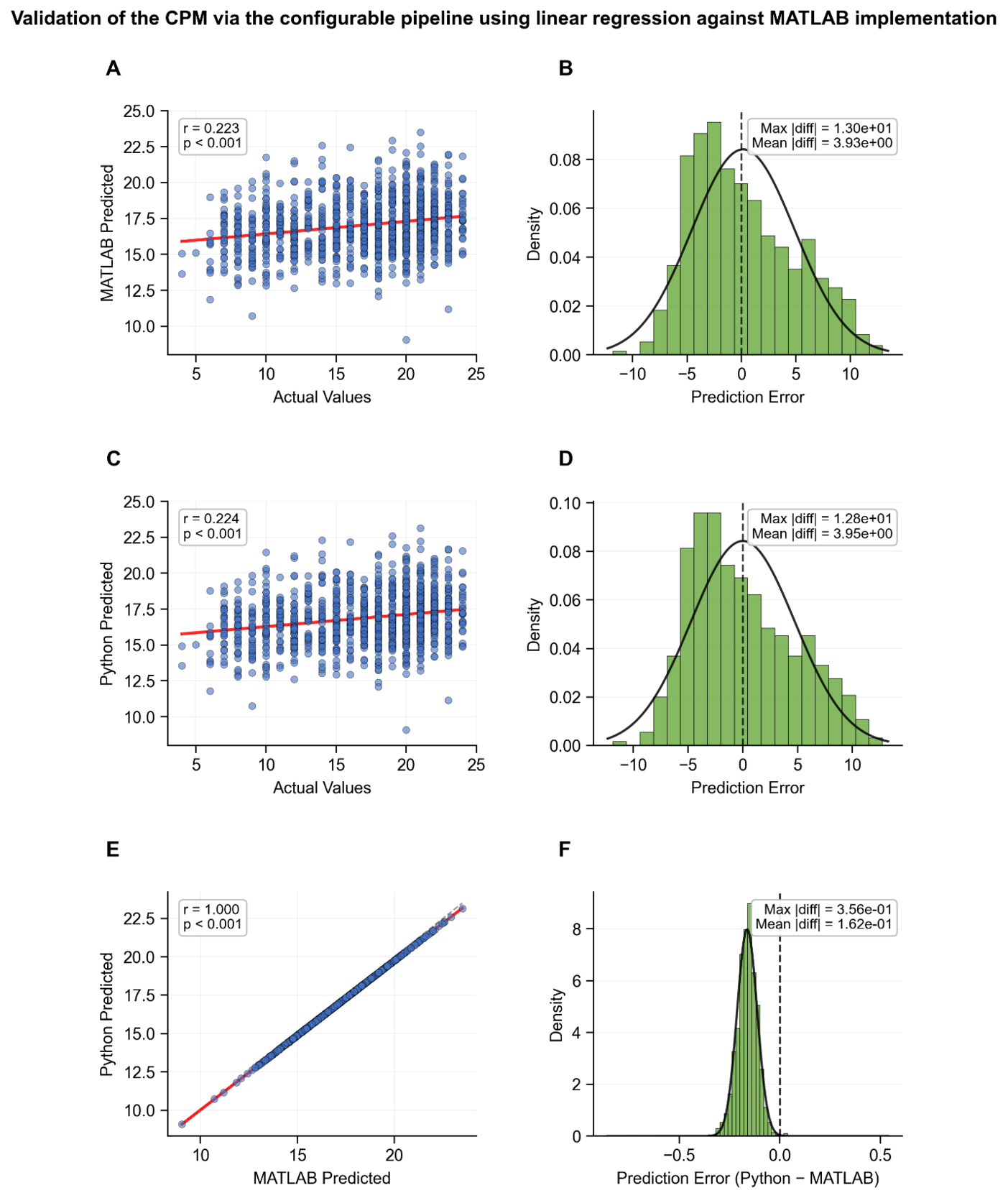
Figure 5 presents the results using our robust regression wrapper: the original MATLAB implementation (panels A–B; r = 0.223, p < 0.001, max |diff| = 1.30e+01, mean |diff| = 3.93e+00) and our configurable pipeline (panels C–D; r = 0.223, p < 0.001, max |diff| = 1.30e+01, mean |diff| = 3.93e+00) showed equivalent prediction performance. Panels E–F directly compare the predicted values, confirming near-perfect numerical agreement (r = 1.000, p < 0.001, max |diff| = 1.33e-03, mean |diff| = 5.28e-04), with negligible residual differences attributable to implementation-level differences between MATLAB’s robustfit and our wrapper (see Limitations). Using the same data, we additionally used ordinary least squares (scikit-learn’s LinearRegression) in place of the robust regression wrapper, consistent with the ordinary least squares approach used in the Python CPM tutorial by Finn¹⁵ (Figure 6). The MATLAB implementation (panels A–B; r = 0.223, p < 0.001) and our pipeline (panels C–D; r = 0.224, p < 0.001, max |diff| = 1.28e+01, mean |diff| = 3.95e+00) showed comparable prediction performance, with agreement between the two sets of predictions (panels E–F; r = 1.000, p < 0.001, max |diff| = 3.56e-01, mean |diff| = 1.62e-01). The larger residual differences compared to Figure 5 reflect the expected discrepancy between ordinary least squares and robust regression rather than any pipeline error. Together, these results validate the ability of our pipeline to reliably reproduce the standard CPM algorithm, including its characteristic sign-based aggregation into a single summary score followed by a final regression step.

While the CPM protocol describes the final prediction step as a linear model without specifying ordinary least squares or robust regression, the Yale MATLAB implementation uses robust regression and the Python tutorial by Finn uses ordinary least squares.^6,14,15 As both approaches yield comparable predictions in this single-predictor setting (Figures 5–6), users may select either method based on their specific needs; robust regression is more resistant to the influence of outliers, while ordinary least squares assumes homoscedastic, normally distributed residuals. Both are supported by the pipeline: ordinary least squares via scikit-learn’s LinearRegression, and robust regression via the custom scikit-learn compatible wrapper provided in the repository.

Figure 5.Validation of the CPM implementation via the configurable pipeline using robust regression against the original MATLAB implementation. Both implementations used 10-fold cross-validation with identical fold assignments on HCP connectivity data (n = 1067), predicting fluid intelligence from resting-state functional connectivity. The pipeline used a scikit-learn-compatible wrapper of statsmodels’ RLM with Tukey’s bisquare weighting to match MATLAB’s robustfit. (A) MATLAB-predicted versus actual values (r = 0.223, p < 0.001). (B) Distribution of prediction errors for the MATLAB implementation, showing maximum (1.30e+01) and mean (3.93e+00) absolute differences. (C) Pipeline-predicted versus actual values (r = 0.223, p < 0.001). (D) Distribution of prediction errors for the configurable pipeline, showing maximum (1.30e+01) and mean (3.93e+00) absolute differences. (E) Direct comparison of predicted values between the two implementations (r = 1.000, p < 0.001). (F) Distribution of absolute differences between implementations, showing maximum (1.33e-03) and mean (5.28e-04) absolute differences.

Figure 6.Validation of the CPM implementation via the configurable pipeline using linear regression against the original MATLAB implementation. Both implementations used 10-fold cross-validation with identical fold assignments on HCP connectivity data (n = 1067), predicting fluid intelligence from resting-state functional connectivity. The pipeline used ordinary least squares (LinearRegression) while the MATLAB implementation used robust regression (robustfit). (A) MATLAB-predicted versus actual values (r = 0.223, p < 0.001). (B) Distribution of prediction errors for the MATLAB implementation, showing maximum (1.30e+01) and mean (3.93e+00) absolute differences. (C) Pipeline-predicted versus actual values (r = 0.224, p < 0.001). (D) Distribution of prediction errors for the configurable pipeline, showing maximum (1.28e+01) and mean (3.95e+00) absolute differences. (E) Direct comparison of predicted values between the two implementations (r = 1.000, p < 0.001). (F) Distribution of absolute differences between implementations, showing maximum (3.56e-01) and mean (1.62e-01) absolute differences.

PNRS Validation

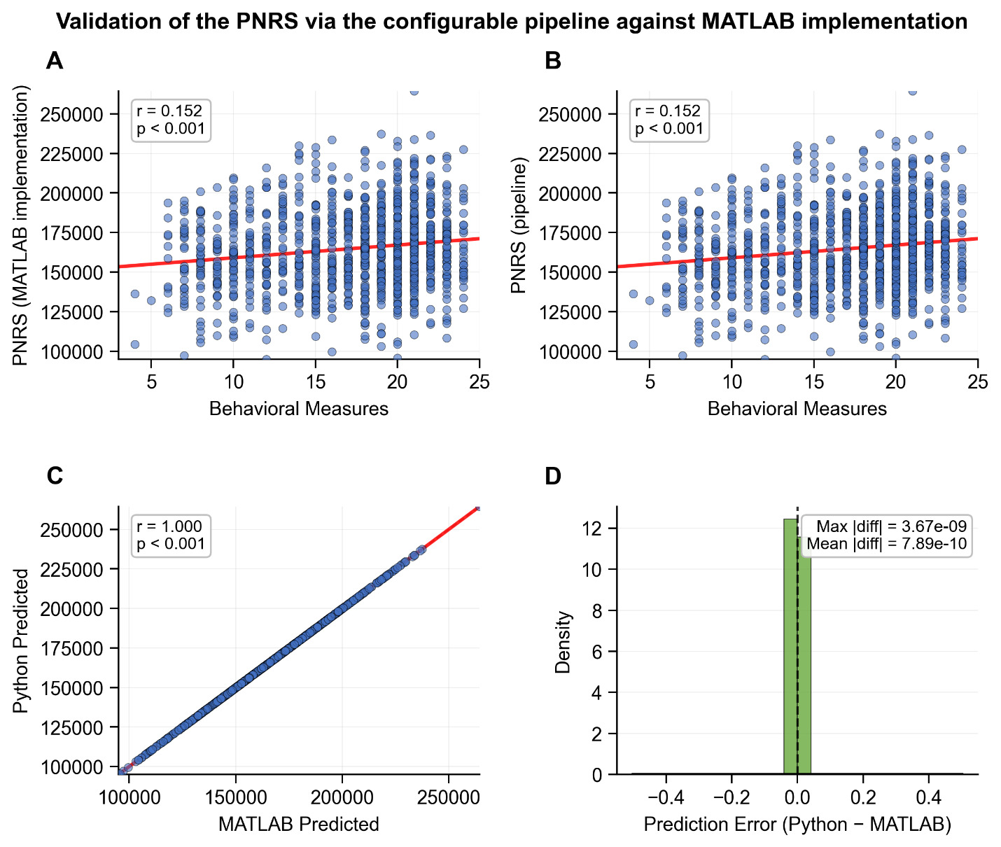
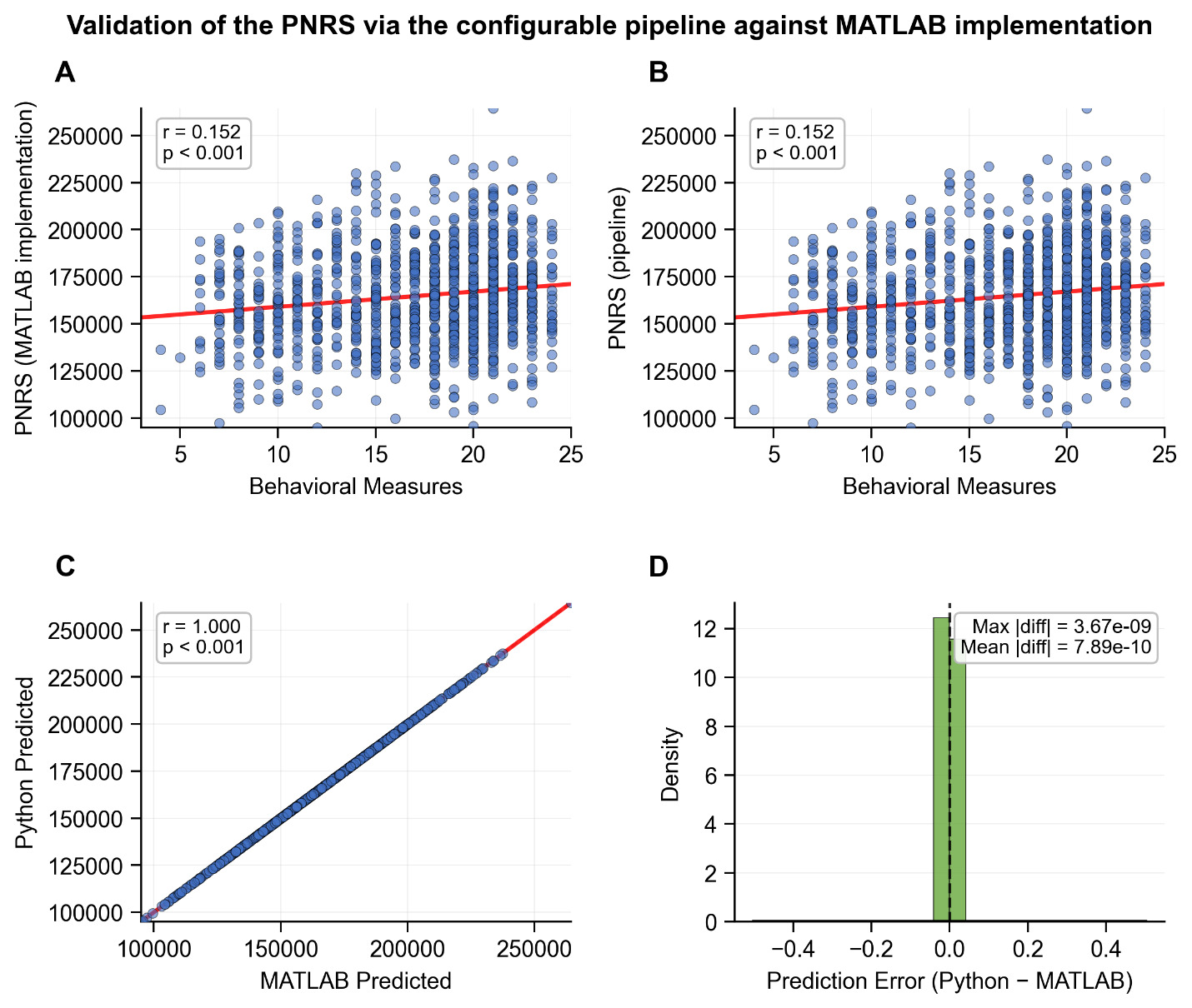
We validated our PNRS implementation against the DCAN Labs BWAS toolbox.^7,16 Using identical in-sample validation on HCP¹⁸ connectivity data (n = 1067), both implementations yielded identical correlation between aggregated scores and behavior. Figure 7 presents the results from the original MATLAB implementation (panel A; r = 0.152, p < 0.001) and our configurable pipeline (panel B; r = 0.152, p < 0.001), showing identical performance. Panels C–D directly compare the PNRS scores of the two implementations, confirming exact numerical equivalence (r = 1.000, p < 0.001, max |diff| = 3.67e-09, mean |diff| = 7.89e-10). These results validate the ability of our pipeline to reproduce the PNRS methodology through appropriate parameter configuration.

Figure 7.Validation of the PNRS implementation via the configurable pipeline against the original MATLAB implementation. Both implementations used identical in-sample validation on HCP connectivity data (n = 1067), computing PNRS scores from resting-state functional connectivity. (A) MATLAB PNRS scores versus actual behavioral values (r = 0.152, p < 0.001). (B) Pipeline PNRS scores versus actual behavioral values (r = 0.152, p < 0.001). (C) Direct comparison of PNRS scores between the two implementations (r = 1.000, p < 0.001). (D) Distribution of absolute differences between implementations, showing maximum (3.67e-09) and mean (7.89e-10) absolute differences, confirming numerical equivalence at machine precision.

PCS Validation

PCS Computation Using an External CSS Matrix

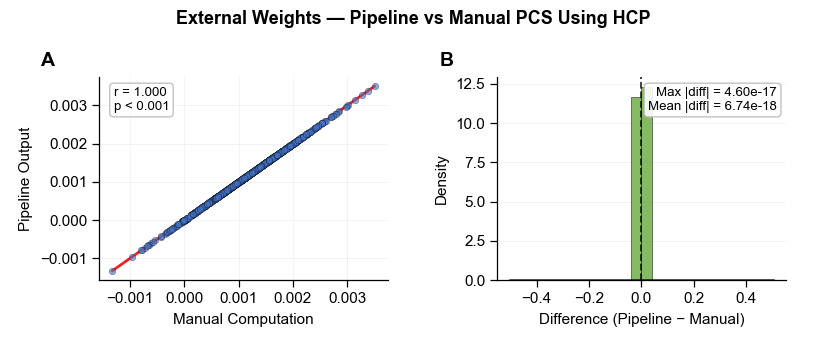
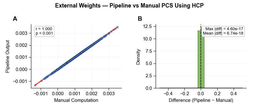
We validated the PCS^8,9 implementation using the external weights workflow with HCP connectivity data¹⁸ and a simulated CSS matrix. Figure 8 presents the correspondence between the pipeline’s PCS scores and those computed directly from the PCS formula (panel A; r = 1.000, p < 0.001, max |diff| = 4.60e-17, mean |diff| = 6.74e-18), confirming exact numerical equivalence (panel B). These results validate the ability of our pipeline to correctly compute PCS using externally derived CSS weights.

Figure 8.Validation of PCS computation with external CSS weights via the configurable pipeline against manual computation. Both approaches used HCP connectivity data (n = 1067) and a simulated CSS matrix. (A) Correspondence between pipeline PCS scores and manually computed PCS scores (r = 1.000, p < 0.001). (B) Distribution of absolute differences between pipeline and manual PCS scores, showing maximum (4.60e-17) and mean (6.74e-18) absolute differences, confirming numerical equivalence.

CSS Derivation for Group Contrasts

We validated the pipeline’s correlation-to-Cohen’s d conversion via the t-statistic derivation^23,24 using two independent approaches. First, we compared the derived CSS values against those computed by the effectsize R package,^25,26 which implements the same r-to-d conversion through the t-statistic. Second, we compared against the Pingouin²⁷ Python library, which computes Cohen’s d directly from group means and pooled standard deviations, providing an independent validation of the conversion pathway itself. Using simulated data with two groups (n₁ = 120, n₂ = 80), Figure 9 presents the correspondence between the pipeline’s CSS values and those from the effectsize R package (panel A; r = 1.000, p < 0.001; panel B; max |diff| = 4.68e-10, mean |diff| = 1.94e-10). Figure 10 presents the correspondence between the pipeline’s CSS values and those from the Pingouin library (panel A; r = 1.000, p < 0.001; panel B; max |diff| = 4.98e-10, mean |diff| = 2.48e-10), confirming that the conversion pathway produces Cohen’s d values consistent with direct computation from group statistics. Together, these results validate our pipeline’s correlation-to-Cohen’s d conversion for group contrast analyses.

Figure 9.Validation of CSS derivation (Cohen’s d) for group contrasts via the configurable pipeline against the effectsize R package. Both approaches used simulated data with two groups (n₁ = 120, n₂ = 80). (A) Correspondence between pipeline-derived and effectsize-derived Cohen’s d values (r = 1.000, p < 0.001). (B) Distribution of absolute differences between the two implementations, showing maximum (4.68e-10) and mean (1.94e-10) absolute differences.

Figure 10.Validation of CSS derivation (Cohen’s d) for group contrasts via the configurable pipeline against the Pingouin Python library. Both approaches used simulated data with two groups (n₁ = 120, n₂ = 80). (A) Correspondence between pipeline-derived and Pingouin-derived Cohen’s d values (r = 1.000, p < 0.001). (B) Distribution of absolute differences between the two implementations, showing maximum (4.98e-10) and mean (2.48e-10) absolute differences.

Runtime Benchmarks

Table 2 reports runtime benchmarks for each pipeline configuration described in the validation section, measuring only the core pipeline computation from input data to final results, excluding data loading and visualization. All benchmarks were obtained on an Intel Core i7 (10th generation) with 8GB RAM.

Illustrative Application: Family-Aware Cross-Validation

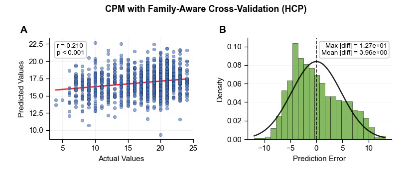
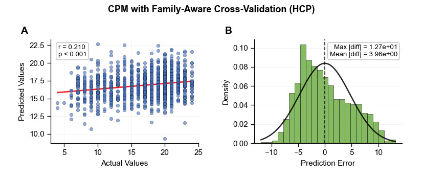
Beyond the validation analyses above, we applied the canonical CPM configuration^6,14 to the HCP data¹⁸ using GroupKFold with each subject’s HCP family ID as the grouping variable, to demonstrate how to use our configurable pipeline for this purpose. Results are shown in Figure 11 (panel A: r = 0.210, p < 0.001; panel B: max |diff| = 1.27e+01, mean |diff| = 3.96e+00). This example illustrates how researchers can integrate family-aware cross-validation into the pipeline for datasets with non-independent observations such as HCP.^20,21

Figure 11.Illustrative application of CPM with family-aware cross-validation on HCP data. Applied to HCP connectivity data (n = 1067) using GroupKFold with HCP family IDs, predicting fluid intelligence from resting-state functional connectivity. (A) Pipeline-predicted versus actual values (r = 0.210, p < 0.001). (B) Distribution of prediction errors, showing maximum (1.27e+01) and mean (3.96e+00) absolute differences

Discussion

The primary contribution of this work is the technical consolidation of MUA methods into a single, standardized, and configurable pipeline. Built within the scikit-learn ecosystem in Python, this unified framework brings together two widely used techniques — CPM⁶ and PNRS⁷ — which we have validated against their original MATLAB implementations,^14,16 alongside PCS^8,9,17 with support for both externally derived and internally computed CSS. Existing implementations of these methods remain fragmented across MATLAB, Python, and R, with no unified framework bringing them together. Furthermore, our pipeline addresses a critical accessibility gap: while the original implementations of CPM and PNRS were developed in MATLAB, which is not open-source, our Python implementation offers a freely accessible alternative, enabling researchers to apply these validated techniques within a modern machine learning framework.

Although different MUA methods share a common computational core, they differ in their specific goals, which our pipeline accommodates through configurable parameters. PNRS⁷ is intended to produce a score that captures the brain-behavior association by evaluating how well the score correlates with the outcome, while CPM⁶ adds a final regression step to produce actual behavioral predictions, as also demonstrated in recent PNRS applications.¹³ Our unified framework supports both: users can work with scores directly or add a final regression step via the ‘regressor’ step in the pipeline, using any scikit-learn-compatible regression method, including the custom robust regression wrapper provided in our repository. PCS^8,9 uses pre-computed CSS matrices to quantify the degree to which an individual’s brain connectivity aligns with disorder- or behavior-related connectivity patterns. As CSS matrices are typically derived from large discovery datasets, users can apply pre-computed CSS from prior studies to assess individual-level connectivity patterns. Our pipeline supports this approach through the external weights option. In addition, users can also derive CSS from a discovery sample within the pipeline itself — using regression-derived β-weights for scale variables or correlation-to-Cohen’s d conversion for two-group contrasts (e.g., patients vs. controls) — supporting the PCS workflow within a single framework.

We validated CPM⁶ and PNRS⁷ against their original MATLAB implementations,^14,16 using HCP data.¹⁸ For CPM, using identical fold assignments, we validated the pipeline with both our robust regression wrapper and ordinary least squares, confirming that the pipeline correctly reproduces the CPM algorithm with either regression method as the final prediction step. For PNRS, the pipeline achieved exact numerical equivalence with the MATLAB implementation. For PCS,^8,9 we validated the external weights workflow against the PCS formula using HCP data, and verified the CSS derivation workflow for two-group contrasts (correlation-to-Cohen’s d conversion) using simulated data against two independent implementations: the effectsize R package^25,26 and Python Pingouin library.²⁷ CSS derivation for scale variables was verified through mathematical equivalence with the validated PNRS regression coefficients. In all cases, the pipeline’s accuracy and correctness were confirmed. By providing comprehensive documentation, validation scripts, and a configurable interface, we aim to minimize implementation errors and enhance reproducibility in neuroimaging research.

MUA-style approaches are preferable to fully multivariate machine learning methods when interpretability and understanding the independent contribution of individual features are of primary interest. In MUA methods, features are selected univariately, and in contrast to fully multivariate models, the model does not learn how to weight features relative to each other. As a result, each feature’s contribution is independently quantifiable and the selected set of connections participating in the model is directly identifiable. This interpretability represents a central advantage of MUA methods, as it enables researchers to determine which specific connections contribute to brain–behavior relationships or play a role in a given clinical symptom.^2,32

However, aggregation-based approaches may be suboptimal in several scenarios: when the relevant brain–behavior relationship depends on interactions between features that cannot be captured by independent evaluation³³; when selected features have unequal predictive importance but are combined with equal contributions²; and when the signal is subtle and distributed, as stringent multiple comparison corrections required by univariate selection may lead to loss of statistical power and information.^33,34 In such cases, fully multivariate methods capable of modelling higher-order dependencies between features may offer improved predictive accuracy and better generalization to independent datasets. However, in fully multivariate models, individual feature weights do not directly reflect the underlying neural sources of an effect due to feature correlations and suppressor variables, making interpretation considerably more challenging.^32,35,36

Therefore, the choice between these approaches should be guided by the specific research question and the relative priority placed on interpretability versus predictive performance. MUA approaches are better suited for establishing transparent, reproducible baselines with direct neurobiological interpretability, while fully multivariate methods may be preferred when maximizing prediction accuracy is the primary objective.

Recommendations & Future Work

For optimal results using our configurable pipeline, we recommend following standard machine learning best practices: (1) ensuring adequate sample sizes based on recent neuroimaging guidelines^1,2; (2) running the “Preprocessing” script available in our repository, which helps to remove faulty subjects; (3) carefully selecting method parameters aligned with research objectives; (4) using group-aware cross-validation whenever observations are non-independent — including related subjects, multi-site data, and repeated measures — to prevent data leakage and inflated performance estimates^20,21; and (5) comprehensively reporting all methodological details.

While our current implementation reliably reproduces established MUA methods, including CPM⁶ and PNRS,⁷ the parameterized configurable pipeline opens exciting possibilities for methodological innovation. Future work will systematically characterize performance across the full parameter space, exploring hybrid configurations such as: (1) combinations of weighting methods (e.g., correlation-based weights for feature selection with regression weights for aggregation); (2) ensemble approaches that combine predictions from multiple parameter configurations; (3) formal runtime benchmarks and memory profiling on large-scale connectome datasets to provide practical guidance.

Conclusion

Our pipeline significantly simplifies the reporting process; users can achieve full methodological transparency by directly documenting the specific input parameters passed to the function. By utilizing these built-in parameters to define the MUA class, standardization, and cross-validation strategy, researchers can seamlessly provide the documentation necessary for exact reproducibility and cross-study comparisons.² By providing this unified platform with comprehensive parameter control, which facilitates application of validated MUA methods and systematic exploration of the MUA design space using standardized machine learning toolkits, this pipeline is intended to provide a more usable, standardized foundation for advancing our understanding of brain-behavior relationships.

Limitations

We note that the HCP dataset¹⁸ includes twins and siblings, which may introduce non-independence among observations. To prevent data leakage when applying these methods to related-family data, users should use family-aware cross-validation strategies (e.g., scikit-learn’s GroupKFold where family ID is the grouping variable; see the Cross-Validation Strategy subsection and the Illustrative Application: Family-Aware Cross-Validation subsection for examples using our configurable pipeline).^20,21 In our validation, we replicated the original studies’ cross-validation schemes (which did not account for family structure) to ensure direct numerical equivalence; however, we strongly recommend family-aware splitting for independent applications. The magnitude of the effect of family-aware cross-validation on prediction performance varies across datasets, outcomes, and modeling choices. Prior work suggests that family-related leakage has relatively minor effects compared to other forms of leakage, though these effects become more pronounced as the proportion of multi-member families increases; users should therefore evaluate this consideration in the context of their own data and pipeline.

For the CPM validation, the Yale MATLAB implementation uses robust regression (robustfit) for the final prediction step.^6,14 As no existing Python package exactly replicates MATLAB’s robustfit, we created a scikit-learn-compatible wrapper using statsmodels’ Robust Linear Model (RLM) with Tukey’s bisquare weighting function (tuning constant = 4.685).³¹ Both implementations use iteratively reweighted least squares (IRLS) with median absolute deviation (MAD)-based scale estimation and share the same default tuning constant. The numerical differences (max |Δβ| = 1.33e-03; Figure 5) between the two implementations remain, attributable to the absence of leverage-corrected residuals in statsmodels’ scale estimation, differences in scale updating procedures across iterations, and convergence criteria. Specifically, MATLAB’s robustfit adjusts residuals by the hat matrix diagonal before computing the MAD scale, whereas statsmodels’ RLM computes the scale from unadjusted residuals. The magnitude of these differences may vary depending on sample characteristics such as sample size and the presence of outliers; however, here, these differences are negligible relative to the effect sizes reported and do not affect the interpretation of results.

For PCS validation, while real CSS matrices are available,^8,9,17 we lacked access to CSS data that matched our specific parcellation scheme (Shen268 atlas³⁰). Therefore, we validated the PCS computation using a simulated CSS matrix and confirmed that our pipeline’s output matched the direct PCS formula with perfect numerical agreement (r = 1.000). Users can apply their own externally derived or internally computed CSS matrices using the same workflow demonstrated in this paper. Additionally, the pipeline’s built-in correlation-to-Cohen’s d conversion computes unadjusted effect sizes for two-group contrasts; however, CSS matrices from prior PCS studies were sometimes derived using Cohen’s d corrected for covariates such as age, sex, and in-scanner motion.^8,9 For datasets requiring confound correction, multi-group contrasts, or other custom CSS for PCS computations, users can derive weights externally and supply them via the external_weights parameter.

Data availability

All raw data used in the present study have been made publicly available by HCP in accordance with data use and access regulations set by the HCP.¹⁸ The Northeastern University and Yale University Human Research Protection Programs approved secondary analyses of these datasets. Human Connectome Project (HCP) data are available through the HCP repository (https://www.humanconnectome.org/study/hcp-young-adult). Users must agree to data use terms before accessing ConnectomeDB; details are provided at https://www.humanconnectome.org/study/hcp-young-adult/data-use-terms.

Code availability

All code used for running statistical analyses has been made publicly available on GitHub at https://github.com/neuroprismlab/_MUA_Pipeline. The BioImage Suite command line software used for processing is freely available at (https://bioimagesuiteweb.github.io/webapp/index.html).

Acknowledgements

This work was supported by funding from the National Institute of Mental Health (R00 MH130894 to S.N). Data were provided by the Human Connectome Project, WU-Minn Consortium (Principal Investigators: David Van Essen and Kamil Ugurbil; 1U54MH091657) funded by the 16 NIH Institutes and Centers that support the NIH Blueprint for Neuroscience Research; and by the McDonnell Center for Systems Neuroscience at Washington University.

Contribution statement

S.N. conceived of the study. F.D. wrote all code and performed all analyses and interpretation under the guidance of S.N. F.C. provided additional guidance on code implementation, and H.S. assisted in final packaging of the pipeline for release. F.D. wrote the manuscript with input from all co-authors.