Automatic detection of simulated artifacts on T1w magnetic resonance images: Comparing performance of different QC strategies

1. Introduction

Magnetic resonance imaging (MRI) is a powerful, non-invasive diagnostic tool that provides detailed images of brain anatomy, making it invaluable for investigating neurological conditions in both research and clinical settings. T1-weighted (T1w) images are frequently used to derive conventional measures of brain health, such as gray matter volume or cortical thickness. However, the reliability of MRI derivatives is heavily dependent on the quality of the acquired MRI scans. Poor image quality not only makes it challenging for radiologists to discern relevant anatomical detail but may also compromise the accuracy and precision of automated image analysis algorithms.^1–4 Therefore, robust quality control (QC) measures are essential to identify and appropriately manage poor-quality images that could negatively impact statistical power in research studies. Beyond guiding exclusion decisions, QC metrics can also be used to modulate confidence in results, serving as covariates or weights in subsequent analyses.^5,6

Traditional QC methods typically involve visual inspection by radiographers, radiologists, or researchers, which is both time-consuming and subjective.^7,8 In contrast, automated QC could offer significant advantages, such as improved reproducibility and standardization by eliminating human bias, and increased efficiency because of computer speed and parallelization potential. These advantages make automated QC a feasible solution for large research studies or potentially even real-time feedback on the scanner in the future. Despite these benefits, the implementation of automated QC has yet to be standardized across institutions, in part due to the diversity of research protocols, scanner hardware, and study aims. Research groups often develop their own QC algorithms to assess image quality, particularly focusing on artifact detection before further post-processing.^9–11 Some of these algorithms are fully automated in performing the assessment (automatic QC), while others still require human intervention at key points (semi-automatic QC). As the field advances, establishing consensus on systematic QC approaches is essential for enhancing the reliability of studies and improving comparability across different research centers and clinical settings.

Semi-automatic and automatic QC algorithms can be categorized into three categories: rule-based (RB), classical machine learning (ML), and deep learning (DL) approaches.¹¹ RB approaches establish thresholds for predefined image quality features, such as signal-to-noise ratio (SNR), to flag scans that fall outside these thresholds.¹² ML algorithms rely on similar predefined features but involve the training of classifiers to differentiate image quality levels.¹⁰ DL algorithms differ from RB and ML as DL does not rely on predefined quality features but instead uses all available image information to classify the images.^13–15

Algorithms from each of these categories have demonstrated high accuracy within (mostly) single-cohort studies, which makes it challenging to compare QC studies due to variations in MRI scanner hardware, MRI protocols, and patient populations.¹⁶ The variability introduced by these factors can lead to discrepancies in image characteristics that are not accounted for by the algorithms trained on a specific dataset. Moreover, the relative performance of these methods is difficult to quantify, as reported accuracy is often contingent on the specific context of the studies and local practices, rather than on universally applicable quality criteria.¹¹ The lack of standardized benchmarking datasets and evaluation metrics further complicates the comparison of different QC methods. For example, some studies may emphasize sensitivity to certain artifacts over others, such as blurring, noise, head motion, or ghosting, which can bias the reported performance metrics.¹⁷

A main challenge in automatically detecting (subtle) artifacts lies in the fact that only a small subsection of MRI scans contains severe artifacts, which are often not shared publicly. On the other hand, most MR images may contain subtle artifacts, which are not detected visually but may already affect statistical power. Simulated artifacts may help in understanding the effects of subtle artifacts, although these are restricted in real-world generalizability.

As a proof of concept, the present study compares the ability of automatic QC algorithms to detect simulated artifacts. The present study focused on a single, standardized T1w MPRAGE protocol from the Alzheimer’s Disease Neuroimaging Initiative (ADNI), to provide a controlled benchmark for comparing the performance of automatic QC algorithms under known synthetic artifact types and severities, to better understand their strengths and limitations. We 1) evaluate whether different severity levels of these synthetic artifacts can be detected visually by human readers; 2) compare the artifact detection performance between RB, ML, and DL; and 3) investigate whether image quality metric (IQM) feature importance differs between RB and ML.

2. Methods

2.1. Data inclusion

Data for this study were drawn from the ADNI dataset, a multisite study of older adults with normal cognition, mild cognitive impairment, or Alzheimer’s disease.¹⁸ Acquisition and reconstruction details for the T1w MRI data were obtained from the ADNI MRI Scanner Protocols (https://adni.loni.usc.edu/data-samples/adni-data/neuroimaging/mri/mri-scanner-protocols/) and MRI Pre-processing documentation (https://adni.loni.usc.edu/data-samples/adni-data/neuroimaging/mri/mri-pre-processing/), together with scan-level metadata in the ADNI Image & Data Archive.

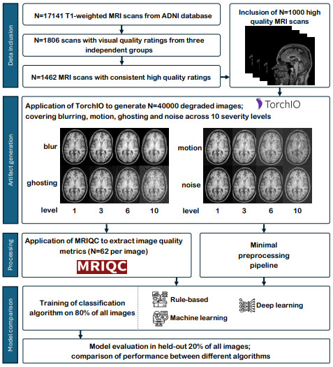
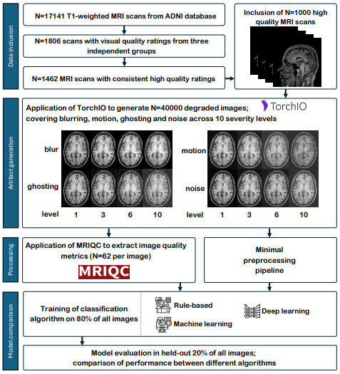
We selected high-quality 3D T1w MRI scans that are free of apparent artifacts, using visual QC scores from three independent groups. From the full pool of 17,141 3D T1w MRI scans¹⁹ (downloaded August 2024), 1,806 3T images had three visual QC scores available for the unprocessed T1w scans, one score from each of the three independent sources: the Dementia Research Centre of University College London (UCL), the NeuroImaging & Surgical Technologies (NIST) Lab of McGill University, and the Public Open Neuroimaging Data Reduction for Artificial Intelligence (PondrAI) QC. The UCL laboratory performed visual QC using a 3-level scale: 1) “ok”, 2) “borderline”, and 3) “fail”. Their assessment focused on identifying the presence of artifacts such as blurring, ghosting, motion, noise, and ringing.²⁰ The McGill laboratory involved 12 raters who performed visual QC using QRater with a 3-level scale: 1) “ok”, 2) “warning”, and 3) “fail”. The QRater visual QC protocol outlines criteria based on coverage, intensity uniformity, motion, and noise.²¹ Finally, PondrAI QC is a public repository containing visual QC of a variety of public datasets. The images were rated by a single rater on a 6-level scale, with 1 indicating good image quality and 6 indicating poor image quality, based on contrast, coverage, noise, and ringing.²²

We rescaled all ratings to a 3-point scale (1–3), with 1 indicating good image quality and 3 indicating poor image quality and summed them to a composite QC score (3–9). A total of 1,462 scans received a composite QC score of 3. Using a fixed random seed, we pseudorandomly selected a subset of 1,000 scans for subsequent analysis (for acquisition details, see Table 1). These 1,000 MRI scans included data from 694 unique participants; 445 participants had only one session, 200 had two sessions, 41 had three sessions, and 8 had four sessions.

2.2. Artifact generation

We added four types of simulated artifacts (blurring, ghosting, motion, and noise) to the 1,000 MRI scans using TorchIO.²³ As TorchIO’s artifact simulations are dependent on image intensities, we normalized the mean and variance of each scan prior to applying the simulations. These normalized images will be referred to as non-degraded images. For each artifact type, we generated ten severity levels (Figure 1) by linearly adjusting the relevant parameters of the TorchIO functions. The lower and upper boundaries for each artifact’s parameter range (sections 2.1–2.4) were defined based on previous work,²⁴ ensuring a clinically realistic spectrum. This approach resulted in 1,000 MRI scans × 4 artifact types × 10 severity levels = 40,000 degraded images, in addition to the 1,000 non-degraded images.

Figure 1.Schematic overview of methods.

2.2.1. Blurring

TorchIO’s RandomBlur function applies a Gaussian kernel to blur the image along each axis.²³ By linearly increasing the standard deviations of the kernels (0.2 to 2), we created various levels of blurring artifact severity.

2.2.2. Ghosting

TorchIO’s RandomGhosting function generates ghosting artifacts by Fourier transforming the image to k-space, creating several shifted copies of the k-space data along a specified axis, scaling these copies by a ghosting intensity parameter, and combining them with the original before inverse Fourier transforming back to the original space. We set the axis to anterior-posterior and linearly increased the ghosting intensity (0.15 to 1.5) for ten severity levels.

2.2.3. Motion

TorchIO’s RandomMotion function simulates rigid-body motion by applying a sequence of random rotations and translations in k-space.^23,25 The interpolation method was set to b-spline, and by linearly increasing both rotation (1 to 10°) and translation parameters (1 to 10 mm) in tandem, we created ten severity levels.

2.2.4. Noise

TorchIO’s RandomNoise function adds zero-mean Gaussian noise without spatial correlation.²⁶ By linearly increasing the noise standard deviations (0.03 to 0.3), we created ten severity levels. If this resulted in voxel intensities below 0, these were retained (no intensity clipping was performed).

2.3. Visual QC of degraded scans

To evaluate how the simulated artifacts relate to those typically observed in real-world scans, we conducted visual QC on a subset of the data using the PondrAI QC rating scale (1 = perfect quality, 6 = terrible quality).²² Three thousand images were randomly selected from the 40,000 degraded images by shuffling the eligible image pool and then selecting the first 3,000, ensuring a representative distribution across all artifact types and severity levels (roughly 75 scans × 4 artifacts × 10 severity levels). Prior to rating, all nine raters completed a standardized training protocol by reviewing the manual provided by PondrAI²² and practicing on a separate set of 100 images randomly selected from the remaining pool (excluding the 3,000 chosen images). A consensus meeting followed the practice session to align interpretations of the rating criteria. Each rater was assigned a subset of 1,000 images such that each image was rated by three raters.

We assessed inter-rater reliability using Krippendorff’s α and the average pairwise Spearman’s rank correlation coefficient (ρ) using R (version 4.4.1; R Foundation for Statistical Computing, Vienna, Austria). Krippendorff’s α was chosen because it is suitable for ordinal data, accommodates missing values, and adjusts for agreement expected by chance, where agreement is indicated as ≥ 0.8 high, 0.67–0.79 moderate and < 0.67 poor.²⁷ Spearman’s ρ was used to quantify the consistency of the relative ranking of images between raters, with correlations indicated as < 0.39 weak, 0.40–0.59 moderate, 0.60–0.79 strong, and ≥ 0.8 very strong.

Krippendorff’s α was computed using the “ordinal” method, with 95% confidence intervals (CIs) estimated via bootstrapping (1,000 iterations). For Spearman’s ρ, all pairwise correlations between raters were calculated for each artifact type using the “pairwise.complete.obs” option to handle missing data, and then averaged.²⁸ Confidence intervals [CI] for Spearman’s ρ were calculated using the Jackknife Euclidean likelihood-based inference approach.²⁹

2.4. Model training

We evaluated three different types of artifact classification algorithms: RB, ML, and DL. For each artifact type and severity level, a separate model was trained to perform binary classification (e.g., the presence vs absence of blurring at severity level 5), resulting in 40 RB models, 40 ML models, and 40 DL models. No combinations of artifacts or severities were trained. All algorithms were implemented using scikit-learn (version 1.2.2).

To prevent data leakage, the data were split at the participant level, with all longitudinal scans from each participant (section 1) assigned exclusively to one set, resulting in a training set of 765 images and a test set of 235 images. Within the training set, 5-fold cross-validation was performed at the participant level: in each fold, 612 images (80% of the training set) were used for model training, and 153 images (20% of the training set) were used for validation, again ensuring that all data from a given participant remained within a single set. For each artifact type and severity level, separate datasets were created, resulting in a total of 40 datasets (4 artifact types × 10 severity levels). All three models were trained independently for each artifact and each severity level, resulting in 120 models.

2.4.1. Input features RB- and ML-based classification models

As input features for the RB and ML-based classification algorithms, we derived IQMs from the 1,000 non-degraded and 40,000 degraded images using MRIQC (version 22.0.1). Briefly, MRIQC performs head motion estimation with AFNI (version 22.0.17),³⁰ followed by brain extraction with SynthStrip (version 1),³¹ tissue segmentation with FSL FAST (version 5.0.11),³² and several image registration steps to MNI space with ANTS (version 2.3.3.dev168-g29bdf),³³ without accounting for dependencies between multiple sessions from the same participant. Subsequently, MRIQC derives a set of 68 IQMs based on the Quality Assessment Protocol.³⁴ The six spatial resolution IQMs (x/y/z matrix size and voxel-size) were excluded because the spatial resolution does not depend on artifacts, resulting in 62 IQMs (Supplementary Table 1).

To distinguish normal from abnormal IQM values, we reuse predefined quality thresholds if they existed in previous literature, which was the case for five IQMs. These reference-based IQMs have a single absolute quality threshold (e.g., intracranial tissue volume fraction).¹⁰ The other 57 non-reference-based IQMs lack established thresholds and are typically used for relative quality comparisons (e.g., SNR).¹⁰ To harmonize vendor-based batch effects among the non-reference IQMs, we calculated the mean and standard deviation for each IQM per vendor in the 1,000 non-degraded images and used these to calculate IQM Z-scores for the 40,000 degraded images.

2.4.2. RB classification model

To develop and evaluate the RB classification model, we applied a multi-stage approach within each cross-validation fold, with the primary goal of determining optimal thresholds at the individual IQM level and then deriving a single threshold to classify the overall image quality. Thresholds for reference-based IQMs were fixed based on previously established values in MRIQC.¹⁰ The non-reference-based IQM thresholds were determined within each training fold by evaluating a range of z-score thresholds for each non-reference IQM (from z = -5 to 5, in increments of 0.05) and selecting the threshold that maximized the Youden Index (YI; [specificity + sensitivity – 1]) in the validation set.¹²

Subsequently, the reference-based IQM thresholds and optimized non-reference-based IQM thresholds were used to binarize IQMs in the training and validation subsets of that fold. Per image, the binary IQM values (1 = good quality; 0 = poor quality) were summed to a compound quality score, ranging from 0 (all IQMs flagged as poor quality) to 62 (all IQMs flagged as good quality). To define the final classification threshold for artifact presence, we used the compound scores from the non-degraded images within the training subset of that fold as a reference and set the cut-off as the mean + 1 standard deviation.

2.4.3. ML-based classification model

The ML-based classification algorithm used nested cross-validation to train and evaluate a random forest classifier (RFC).¹⁰ Model training was performed using five outer folds for feature selection and model evaluation, and five inner folds for hyperparameter tuning.

To focus on the most informative IQMs while minimizing spurious or site-related influences, a two-step feature selection pipeline was applied in each outer fold.¹⁰ First, an extra trees classifier was trained to predict site using all IQMs,³⁵ and the IQMs most predictive of site were removed. Second, a Winnow-based selection was performed to retain only those features that provided more information than a randomly generated feature. Subsequently, this reduced feature set was used to optimize the inner folds hyperparameters.

Within each inner fold, a grid search was conducted to optimize the RFC’s hyperparameters for YI (number of estimators [10, 100, 500], maximum features [2, 4, 6, 8, 10, 15, 20], maximum depth [10, 20, 30, 50], and minimum samples split [5, 10, 20]).

2.4.4. DL-based classification model

Unlike RB and ML-based classification models, which rely on IQMs extracted with MRIQC, the DL classification algorithms were directly trained on minimally preprocessed non-skull-stripped images. To keep the preprocessing comparable between the classification algorithms, we modified an existing preprocessing pipeline¹³ to correspond with the preprocessing of MRIQC. Bias field correction was applied using the N4ITK method,³⁶ and spatial registration to MNI space was performed using ANTs. The minimum and maximum MNI space T1w image values were rescaled to a range ∈ [0,1].

We trained an existing convolutional neural network (CNN) architecture with its original hyperparameters and loss functions,¹³ using five convolutional blocks followed by three fully connected layers. Each convolutional block consisted of a convolutional layer, a batch normalization layer, a rectified linear unit, and a max pooling layer. This CNN previously demonstrated the best performance for MRI QC in a large heterogeneous clinical dataset.

2.5. Final model evaluation

For all 120 models, the configuration (e.g., thresholds, hyperparameters, model weights) achieving the highest YI across all five folds was selected. Notably, for ML-based classification, this involved the outer folds of the nested cross-validation procedure. Subsequently, the final model performance of each model was evaluated on the independent test set (n = 235). In addition to our primary performance metric YI, we also calculated accuracy, balanced accuracy, F1 score, precision, and recall to evaluate prediction accuracy.

2.6. Feature importance of RB and ML models

To explore model interpretability of RB and ML algorithms, IQM importance was examined across the artifact types and severity levels. For each of the 80 RB and ML models, the most important IQMs were identified as those with the highest YI in RB models and those retained after feature selection in ML models, and these were recorded across all artifact and severity combinations for the final model.

For interpretation purposes, IQMs are grouped into four main categories: entropy, contrast, inhomogeneity, and normative IQMs.^9–11,34 Entropy IQMs, such as the entropy focus criterion (EFC), capture the randomness or complexity in image intensity distributions. Image contrast IQMs, for example the contrast-to-noise ratio (CNR), quantify the distinguishability between different tissue types or structures. Intensity inhomogeneity IQMs, such as intensity non-uniformity (INU), assess the low frequency spatial uniformity of image intensity. Normative IQMs, including metrics like the overlap of tissue probability maps and the scan segmentations (TPM overlap), compare image characteristics to a reference population or template to detect deviations from expected norms. For each artifact type, Spearman’s rank correlations (⍴) were computed between severity levels (ordinal, 1–10) and IQM values (EFC, CNR, INU, TMP). ⍴ values were interpreted according to the following bins: negligible (< |0.10|), weak (|0.10–0.39|), moderate (|0.40–0.69|), strong (|0.70–0.89|), and very strong (> |0.90|).³⁷

3. Results

3.1. Dataset characteristics

Demographic characteristics of the study population, including age, sex, and scanner vendor distribution for the 1,000 non-degraded images are summarized in Table 1. Descriptive statistics of the 62 IQMs of these images, stratified by vendor, are provided in Supplementary Table 1.

3.2. Visual QC ratings across simulated artifacts

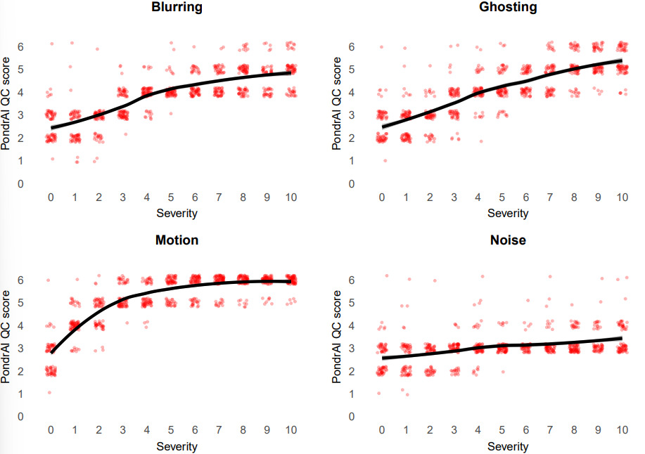
Visual QC ratings increased with artifact severity for most artifact types (Figure 2). Overall, higher simulated artifact severity was associated with higher QC ratings. Blurring and ghosting showed a trend of linear increase across severity levels, indicating that simulated severity corresponded well to the PondrAI QC rating scale (i.e., higher artifact severity was associated with poorer image quality). For motion, ratings reported a logarithmic trend, with intermediate motion severities already scoring high on the PondrAI QC scale. Noise showed only a slight upward trend, with most ratings remaining between 2 and 4.

Figure 2.Visual QC ratings based on the PondrAI QC scale (Costantino and Devenyi, 2023) as a function of artifact severity (0–10) for four artifact types: blurring, ghosting, motion, and noise. Red dots show individual ratings; black lines show smoothed trend lines with 95% confidence intervals, computed using locally estimated scatterplot smoothing. Blurring and ghosting display an approximately linear increase in QC ratings with severity, motion shows a ceiling effect, and noise shows minimal change.

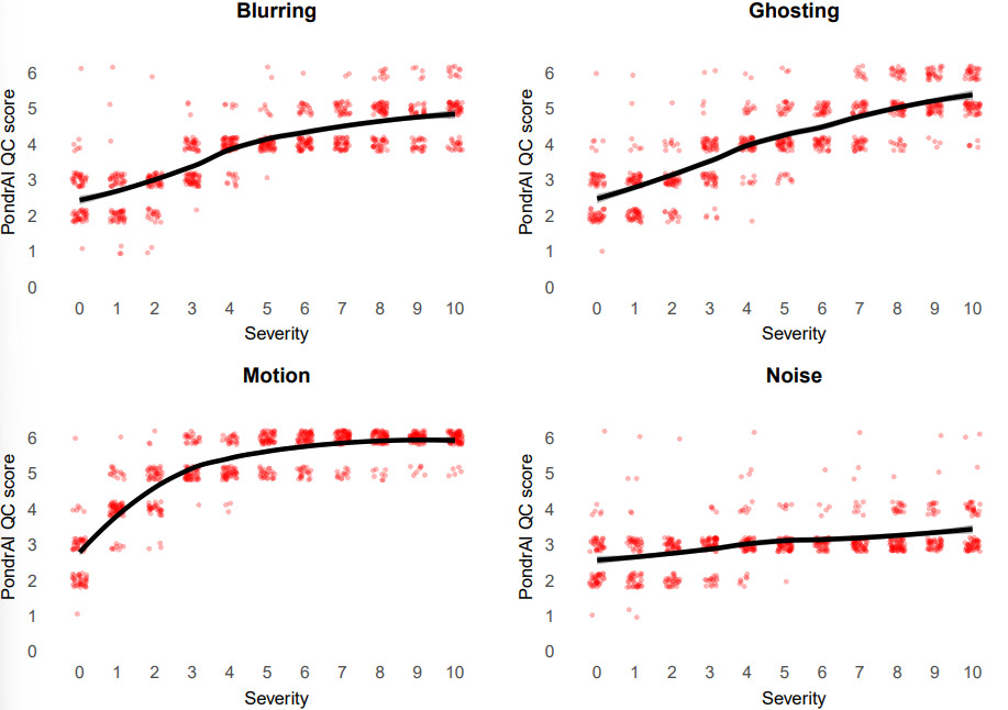
While inter-rater reliability was strong when assessed across all artifact types (α = 0.82, 95% CI: 0.81–0.83; mean ρ = 0.87, 95% CI: 0.84–0.90), it varied considerably between individual artifacts. Ghosting showed the highest agreement (α = 0.79, 95% CI: 0.77–0.82; mean ρ = 0.84, 95% CI: 0.76–0.92). Blurring and motion had poor agreement based on Krippendorff’s α (0.63, 95% CI: 0.59–0.66 and 0.54, 95% CI: 0.49–0.58 respectively), but still relatively high consistency in ranking (mean ρ = 0.77, 95% CI: 0.65–0.88; mean ρ = 0.73, 95% CI: 0.57–0.88 respectively). For both noise and non-degraded images, reliability was lower, with Krippendorff’s α values of 0.41 (95% CI: 0.35–0.46) and 0.31 (95% CI: 0.13–0.45) and lower mean Spearman’s ρ values (0.46, CI: 0.26–0.70 and 0.32, CI: 0.55–0.87, respectively), indicating less agreement in both scores and image ranking. These differences are further illustrated in the pairwise Spearman’s ρ heatmaps (Supplementary Figure 1).

3.3. RB, ML, and DL model comparisons

Detailed RB-, ML-, DL-based classification results for blurring, ghosting, noise, and motion and severity levels 1–10 are shown in Table 2. In terms of computational time, once IQMs had been extracted or the preprocessing had been completed and algorithms were trained, RB, ML, and DL algorithms required approximately  19 ± 6 ms, 3 ± 4 ms, and 2 ± 1 ms per scan, respectively.

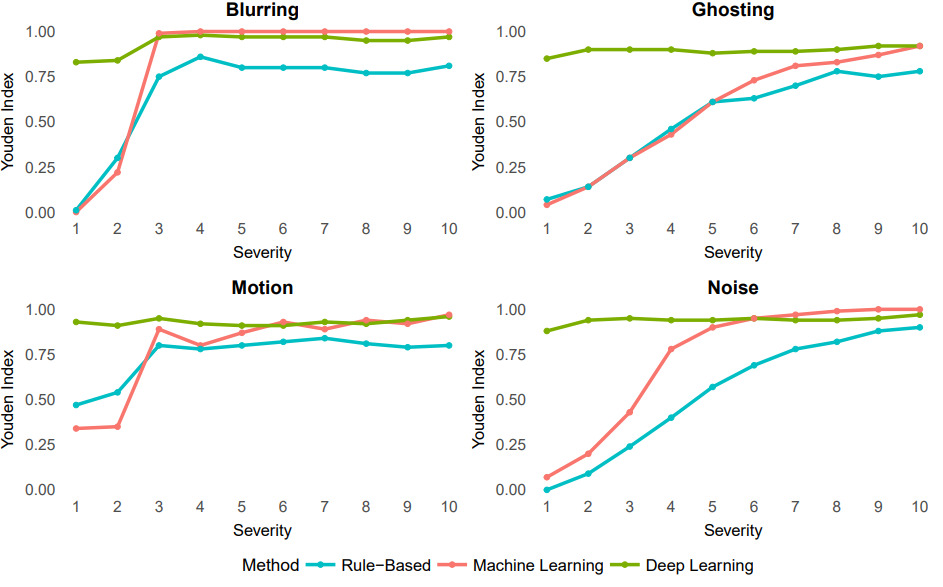
For blurring, DL-based classification demonstrated strong discrimination across all severities (YI = 0.83–0.97, Figure 3). RB classification showed a strong upward trend, especially at severity 3, with YI rising from 0.30 to 0.75 and continuing to improve to very strong performance (YI = 0.81) at the highest severity. ML-based performance was also initially weak with YI = 0 at severity 1, but improved rapidly, reaching near-perfect levels (YI ≥ 0.99) by severity 3. For ghosting, DL models maintained strong discrimination (YI 0.85–0.92) across all severities, while both RB and classical ML models showed weak discrimination at early severities (YI < 0.15), improving to strong (YI = 0.78) and very strong (YI = 0.92) discrimination, respectively, at maximum severity. For motion, DL based classification achieved consistently very strong YI (0.91–0.96), while RB models showed moderate discrimination at low severity (0.47), improving to 0.80 at severity 10, and classical ML based models exhibited a similar trend but with higher maximum performance (YI = 0.97). In the case of noise, DL classification maintained strong performance with YI between 0.88 and 0.97, outperforming both RB and ML models at lower severities; classical ML reached perfect discrimination (YI = 1.00) at higher severities, whereas RB models improved gradually from 0.00 to 0.90.

Figure 3.Youden Index scores across artifact severity levels (1–10) for each artifact type (blur, ghosting, motion, and noise), comparing performance of rule-based (blue), machine learning-based (red), and deep learning-based (green) classification methods. Each panel presents results for a single artifact type. Lines represent the Youden Index (sensitivity + specificity – 1) at each severity level.

Overall, these findings indicate that DL-based classification is consistently robust across all artifact types and severities, while RB and ML models are more reliably performant only at higher levels of artifact severity and show limited discrimination accuracy at lower severities across all artifact types. Other evaluation metrics, displaying the same trends as the YI, are shown in Supplementary Figures 2–6.

3.4. IQM importance for RB- and ML-based classification

IQMs exhibited distinct patterns across artifact types and severity levels (Supplementary Figure 7, Supplementary Table 2). For blurring, there were moderately increased values of EFC (⍴ = 0.68) and CNR (⍴ = 0.56), and a weak positive association for TPM (⍴ = 0.33), alongside a weak negative association for INU (ρ = -0.24), indicating greater image entropy, enhanced contrast, and tissue probability map distortion at higher severities. Ghosting led to weak increases in INU (ρ = 0.35) and weak declines in TPM (ρ = -0.31), while EFC and CNR remained relatively stable (ρ = -0.15 and ρ = 0.05, respectively), suggesting spatial misalignment without major changes in contrast or entropy. Motion was associated with weakly increasing INU (ρ = 0.34) and moderately decreasing TPM (ρ = -0.42), reflecting spatial distortion and misclassification of tissue classes, while EFC and CNR remained stable. In contrast, noise resulted in declines in EFC (ρ = -0.71) and moderate increases in INU (ρ = 0.50), while showing negligible-to-weak declines in both CNR (ρ = -0.21) and TPM (ρ = -0.14). These trends highlight the complementary sensitivity of EFC, CNR, INU, and TPM to different artifact types and intensities (Supplementary Figure 7).

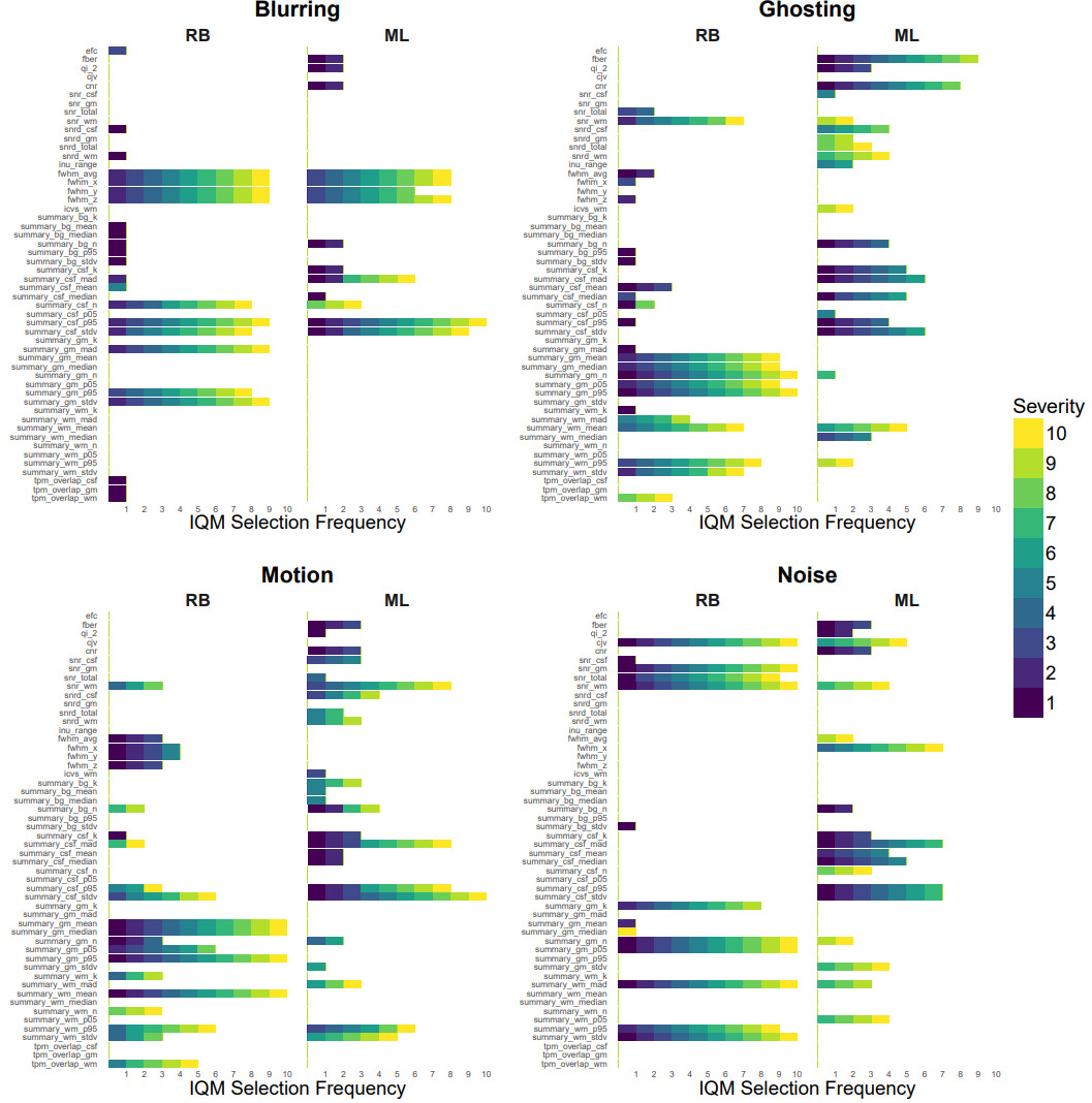
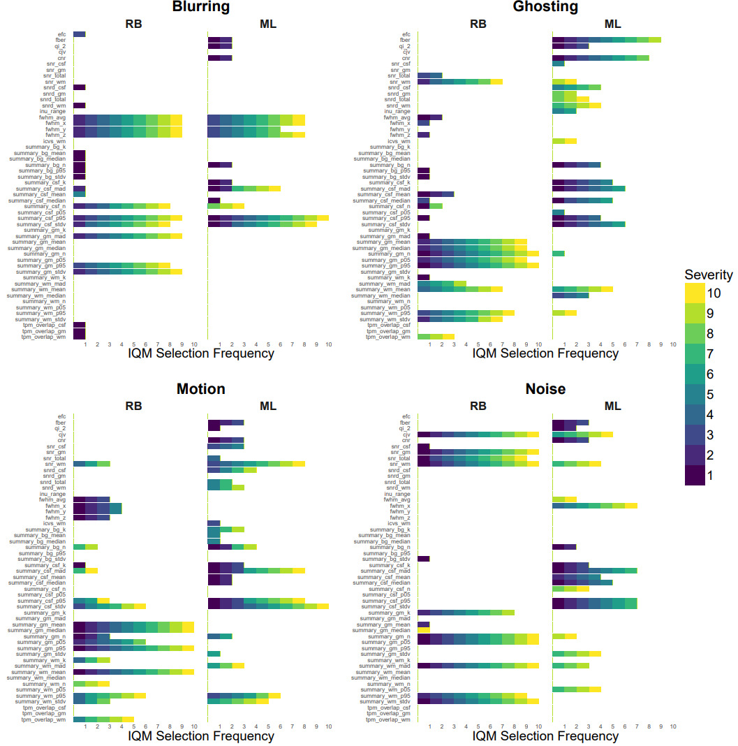
The pattern of IQM selection across artifact types and severity levels for the RB and ML-based classification is displayed in Figure 4. For blurring, both ML and RB models initially selected a broad mix of normative and entropy IQMs, alongside some image contrast IQMs. From severity level 3 onward, RB and ML models consistently prioritized normative and entropy IQMs, particularly those reflecting spatial properties and deviations in cerebrospinal fluid (CSF), while rule-based models reduced their selection to a smaller set of normative features, mainly related to CSF and spatial structure. For ghosting, RB models relied mainly on normative IQMs related to the gray matter and white matter, and a few image contrast IQMs. ML models relied at lower severities mainly on normative IQMs related to the CSF, while at higher severities it shifted to normative IQMs related to the white matter, and some image contrast IQMs. For motion, both RB and ML models initially used normative IQMs. However, RB models’ most informative normative IQMs were related to gray matter, white matter, and CSF, whereas ML models used mainly background related normative IQMs. At higher severities, the most informative IQMs for RB models were the normative IQMs. ML models relied on the GM and background related normative IQMs and SNR-related image contrast IQMs. For noise, ML models initially drew from all four categories but shifted toward normative IQMs, particularly those reflecting CSF, gray matter, and entropy measures (full width at half maximum related). In contrast, RB models narrowed their focus more abruptly, retaining mainly normative (GM related) and image contrast (SNR related) IQMs.

Figure 4.Frequency of IQM selection across artifact types, severity levels and classification models. Each panel shows the number of models (x-axis) that selected each IQM (y-axis) for a given artifact type (blur, ghosting, motion, noise), separately for rule-based (RB) and machine learning-based (ML) classification. Color indicates artifact severity (1–10). As the deep learning-based classification models did not have input features, they are not shown in this figure.

4. Discussion

This benchmark study yielded three main findings. First, while visual QC ratings correlated with simulated artifact severity, the non-linearity of these relations varied between the artifacts. Second, while there was little performance difference for detecting high severity simulated artifacts, DL outperformed RB and ML for detecting subtle simulated artifacts. RB and ML performed similarly, with performance varying between artifact types. Third, RB models relied mainly on a consistent core of normative features with limited use of contrast measures, whereas ML models adapted their feature use depending on artifact type and severity, drawing more flexibly from multiple IQM categories.

Our findings highlight that human visual QC is not equally effective across artifact types, which may have important implications for its use as a benchmark. The high inter-reader agreement for ghosting suggests that artifacts of this type can be reliably perceived. For blurring and motion, inter-rater agreement was lower but individual raters’ assessments remained relatively monotonic with respect to the simulated level of the artifact. Noise, in particular, was rated differently by different readers, perhaps reflecting its weaker perceptual salience, or limited noise variability in the higher severities of the PondrAIQC training examples. Another potential explanation for the relative insensitivity of human raters to noise is that they can consistently interpret detail in an image obscured with noise.³⁸ These findings are in line with previous studies. When comparing human visual QC with machine-based, non-artifact specific, QC scores, previous studies also found poor correspondence, particularly for subtle or borderline real-world artifacts.^39,40 Another study with synthetic artifacts found stronger correlations of radiologist diagnostic quality scores with perceptually aligned image quality metrics, such as DISTS and HaarPSI, than with other IQMs.⁴¹ Together, this highlights the limitations of visual QC as a gold standard for subtle (synthetic) artifacts, whether for detecting general image quality or for detecting specific artifacts.

The fact that DL mostly outperformed RB and ML at low artifact severities aligns with previous studies, which suggest that DL architectures can learn more complex hierarchical image representations and more subtle textural and structural deviations than traditional image features.^13–15,42 Within our benchmark, this advantage seems especially pronounced for simulated artifacts with distributed, non-local changes in image intensity and spatial coherence, such as the simulated ghosting and motion.^10,43 Nevertheless, RB and ML approaches remained highly effective in detecting simulated blurring and noise artifacts, especially at higher severity levels, where degradation can be more easily captured by single or composite IQMs.^12,44 In line with this, it has been shown that, in head-to-head comparison, classical ML models trained on robust IQMs can match DL models for motion artifacts.⁴⁵ Together with these studies, our findings suggest that simpler ML models might offer an alternative to DL, which can be beneficial as they can be more efficient and easier to implement, especially when the goal is to merely detect gross artifacts.

The importance of IQMs for simulated artifact detection by RB and ML varied with the simulated artifact type and severity. At low artifact severities, both RB and ML relied on a broad spectrum of normative and image contrast IQMs to detect subtle or diffuse degradations. With increasing severity, the IQM selection consistently shifted toward normative features, particularly those quantifying deviations from the expected anatomical patterns and spatial properties. Similarly, previous studies demonstrated that global entropy and contrast IQMs are sensitive to early or mild artifacts,^9,44,46 while normative, region-based IQMs offer superior sensitivity and specificity for more severe or localized degradations.^10,39 The increasing reliance on normative IQMs when using simulated artifacts might be relevant in large neuroimaging studies, where heterogeneity in acquisition and (physio-)pathology can obscure subtle artifacts unless deviations from normative patterns are explicitly modeled.^9,10,40 However, it remains to be established the same feature-selection patterns occur for real-world artifacts.

A key strength of our study is the use of synthetic artifacts for benchmarking, which allows for precise control over artifact type and severity, and the ability to generate large, balanced datasets for model training and evaluation.^23,24 However, these simulations should be regarded as controlled approximations rather than realistic reproductions of real-world MRI artifacts, as the simulations do not capture the heterogeneous and subtle degradations that arise from the complex interactions between head motion, hardware imperfections, and acquisition parameters.^42,47 In particular, the artifacts were simulated on magnitude-only reconstructed images rather than using complex-valued raw k-space data. Consequently, the simulations do not reproduce the full interaction between acquisition-time artifacts, coil sensitivities, channel combination, parallel-imaging reconstruction, and vendor-specific preprocessing. Our simulated motion uses simplified perturbations of image-derived k-space and does not model motion confined to subsets of k-space, so it captures only a subset of motion-artifact phenotypes. Similarly, the simulated ghosting is generated as shifted copies of the signal along a single axis and does not include reconstruction-related failures or all aliasing-like patterns. For blurring, a Gaussian image-space blur cannot represent all real-world sources of blurring. The simulated noise is additive, zero-mean Gaussian noise without spatial correlation and therefore does not reproduce the spatially varying, non-Gaussian noise that can result from multichannel reconstruction and vendor preprocessing. We did not validate the results based on simulated artifacts against independently labelled real-world motion, noise, ghosting, or blurring artifacts. Therefore, the present findings establish performance only under the specific simulated artifacts used here and cannot be assumed to generalize to real-world artifacts.

The ADNI preprocessing and reconstruction pipeline includes gradient-nonlinearity distortion correction, B1 and N3 intensity normalization, phantom-based spatial scaling, and vendor-applied gradient-linearity and B1-corrections (https://adni.loni.usc.edu/data-samples/adni-data/neuroimaging/mri/mri-pre-processing/). These steps improve geometric and intensity homogeneity but place our simulations in a preprocessed image-space domain rather than in the native acquisition domain. Therefore, image-space simulations such as blurring, ghosting, motion, and noise may differ from corresponding artifacts as they arise in real-world raw k-space, and the effects of the ADNI reconstruction and preprocessing pipeline may have removed, attenuated, or transformed artifact characteristics before simulation. This aligns with broader concerns in MRI benchmarking where the use of processed or simplified data can produce inflated performance estimates and reduced generalizability to real raw acquisitions.⁴⁸ As a result, the algorithms we trained on our synthetic artifacts may have partially exploited regularities introduced by the simulation pipeline itself, rather than fully capturing the heterogeneous and subtle degradations typically observed in real-world artifacts, and therefore we cannot determine whether the relative performance of RB, ML, and DL would be preserved when detecting real-world artifacts in images produced by different acquisition and reconstruction pipelines.

Moreover, real MRI scans often exhibit multiple, overlapping artifact types that can impact image quality simultaneously, perhaps often at too-low severities to be visible to the human eye. We chose only to compare the detectability of individual simulated artifacts to maximize interpretability. With the present data, we cannot determine how the interaction of multiple artifacts would interfere with the detection of a single specific artifact, nor whether such interference matters if the primary goal is to assess overall image quality rather than identify a specific artifact type. The models may behave differently when artifact types interact. For these reasons, our conclusions are restricted to the relative performance of QC strategies in detecting individual synthetic artifacts on ADNI T1w MPRAGE scans, and therefore the performance metrics reported should be interpreted as characterizing relative behavior within this controlled benchmark and should not be reused quantitatively for clinical QC deployment without further validation.

Recent work employed transfer learning to retrain DL models on small sets of real, artifact-labeled images after pretraining on synthetic artifacts,²⁴ showing that this combination of simulated and real-world artifacts leads to higher artifact detection performance and generalizability. Although this combination of simulated and real-world artifacts led to higher performance and generalizability, it does not allow disentangling the presence of individual artifacts. Automatic disentangling between artifact types may have value to differentiate scanner and sequence stability from patient compliance. Together, these findings suggest that future research should employ advanced explainable DL algorithms, trained with a combination of individual synthetic artifacts and real-world artifacts.

Another factor limiting the generalizability of our study is the reliance on a single dataset for both training and validation. Although ADNI is a multisite study, its standardized protocols and participant demographics may not fully represent the diversity encountered in clinical practice or other research cohorts.^9,11,16 This homogeneity could inflate model performance and limit its generalizability. Previous studies have highlighted the challenges of cross-site generalization for automated QC, emphasizing the need for diverse, multi-cohort benchmarks and harmonization strategies.^10,42,49 Future studies should prioritize external validation using datasets with real-world artifacts and broader demographic variability.

Furthermore, we prioritized comparability over performance, by employing ML and DL models that were often used and available open-source, with their standard parameter settings from previous studies. While these models ranked among the best-performing approaches for T1w QC,^{10,14,39,40,42} they may be outperformed by more recent and advanced methods, such as a ProtoPNet⁵⁰ or by more extensive hyperparameter optimization or ensemble methods. Additionally, we did not investigate why DL models were more successful at detecting subtle artifacts, as exploring model interpretability (e.g., through saliency mapping, SHAP values, or feature attribution methods),^13,51 was beyond the scope of this study. Systematically benchmarking advanced DL models and integrating explainable AI in future studies could establish the true upper bounds of automated QC performance in neuroimaging.

Finally, the relevance of a QC score and the ability to define a QC threshold may vary between use cases. For example, a radiologist may still find a subtly-degraded image diagnostically usable while it already has lost its potential to show subtle findings in group studies. Training DL models may require different image quality than image-derived phenotypes. Future studies may investigate if QC scores predict the robustness of image-derived phenotypes, affect statistical power, and how automatic QC can be used in clinical practice or trial workflows.

In conclusion, our findings demonstrate that, within this controlled synthetic artifact benchmark, DL offers superior performance for the automated detection of individual synthetic artifacts in T1w brain MRI, particularly for subtle artifacts. RB and ML methods may remain valuable for interpreting quality degradation of artifacts with well-defined quantifiable features. For RB and ML methods, the varying importance of IQMs across simulated artifact types and severities highlight the need for flexible, multi-metric QC frameworks. Future studies should address the challenges of real-world generalizability, model complexity, and interpretability between synthetic and real-world artifacts to fully realize the potential of automated QC in neuroimaging.

Code availability

The code for artifact simulation and the training of the rule-based algorithm is available at the Corresponding author’s GitHub:

https://github.com/janinehendriks-hub/AutoQC-compare-MRI

Acknowledgements

This project was funded by Health~Holland, Top Sector Life Sciences & Health (TKI-PPP Amsterdam UMC 2011227).

Data collection and sharing for the Alzheimer’s Disease Neuroimaging Initiative (ADNI) is funded by the National Institute on Aging (National Institutes of Health Grant U19AG024904). The grantee organization is the Northern California Institute for Research and Education. In the past, ADNI has also received funding from the National Institute of Biomedical Imaging and Bioengineering, the Canadian Institutes of Health Research, and private sector contributions through the Foundation for the National Institutes of Health (FNIH) including generous contributions from the following: AbbVie, Alzheimer’s Association; Alzheimer’s Drug Discovery Foundation; Araclon Biotech; BioClinica, Inc.; Biogen; Bristol-Myers Squibb Company; CereSpir, Inc.; Cogstate; Eisai Inc.; Elan Pharmaceuticals, Inc.; Eli Lilly and Company; EuroImmun; F. Hoffmann-La Roche Ltd and its affiliated company Genentech, Inc.; Fujirebio; GE Healthcare; IXICO Ltd.; Janssen Alzheimer Immunotherapy Research & Development, LLC.; Johnson & Johnson Pharmaceutical Research & Development LLC.; Lumosity; Lundbeck; Merck & Co., Inc.; Meso Scale Diagnostics, LLC.; NeuroRx Research; Neurotrack Technologies; Novartis Pharmaceuticals Corporation; Pfizer Inc.; Piramal Imaging; Servier; Takeda Pharmaceutical Company; and Transition Therapeutics.